AORC Data

DayMet’s API has recently gone down, leading us to experiment with a new type of met data, AORC, which is the dataset used to drive the National Water Model.

%load_ext autoreload
%autoreload 2

AORC provides gridded meteorological data for the conterminous US and Alaska at ~800m spatial resolution with hourly timestep from 1979 (Conterminous US) or 1981 (Alaska) ~ present. website

Available variables:

Variable	Description (units)
APCP_surface	Total precipitation [mm]
DLWRF_surface	Incident longwave radiation flux density [W m^-2]
DSWRF_surface	Incident shortwave radiation flux density [W m^-2]
PRES_surface	Air pressure [Pa]
SPFH_2maboveground	Specific Humidity [g/g]
TMP_2maboveground	Air temperature [°C]
UGRD_10maboveground	West-East component of the wind velocity [m s^-1]
VGRD_10maboveground	North-South component of the wind velocity [m s^-1]

Notes:

• AORC, unlike DayMet, provides all Gregorian calendar days

%matplotlib inline
import matplotlib.pyplot as plt
import matplotlib as mpl
mpl.rcParams['figure.dpi'] = 150

import logging
import numpy as np
import os
import cftime, datetime

import watershed_workflow
import watershed_workflow.ui
import watershed_workflow.sources
import watershed_workflow.meteorology
import watershed_workflow.io

watershed_workflow.ui.setup_logging(1,None)

coweeta_shapefile = 'Coweeta/input_data/coweeta_basin.shp'
crs = watershed_workflow.crs.default_crs

Load the Watershed

coweeta_source = watershed_workflow.sources.ManagerShapefile(coweeta_shapefile, id_name='BASIN_CODE')
coweeta = coweeta_source.getShapes(out_crs=crs)

watershed = watershed_workflow.SplitHUCs(coweeta)
watershed_workflow.split_hucs.simplify(watershed, 60)

Download the raw DayMet raster

returned raw data has dim(nband, ncol, nrow)

startdate = "2010-1-1"
enddate = "2013-12-31"

# setting vars = None to download all available variables
source = watershed_workflow.sources.ManagerAORC()
met_data = source.getDataset(coweeta, start=startdate, end=enddate)

Variable size: 79.2 TB
<xarray.Dataset> Size: 79TB
Dimensions:              (time: 35064, latitude: 4201, longitude: 8401)
Coordinates:
  * latitude             (latitude) float64 34kB 20.0 20.01 20.02 ... 54.99 55.0
  * longitude            (longitude) float64 67kB -130.0 -130.0 ... -60.01 -60.0
  * time                 (time) datetime64[ns] 281kB 2010-01-01 ... 2013-12-3...
Data variables:
    APCP_surface         (time, latitude, longitude) float64 10TB dask.array<chunksize=(144, 128, 256), meta=np.ndarray>
    DLWRF_surface        (time, latitude, longitude) float64 10TB dask.array<chunksize=(144, 128, 256), meta=np.ndarray>
    DSWRF_surface        (time, latitude, longitude) float64 10TB dask.array<chunksize=(144, 128, 256), meta=np.ndarray>
    PRES_surface         (time, latitude, longitude) float64 10TB dask.array<chunksize=(144, 128, 256), meta=np.ndarray>
    SPFH_2maboveground   (time, latitude, longitude) float64 10TB dask.array<chunksize=(144, 128, 256), meta=np.ndarray>
    TMP_2maboveground    (time, latitude, longitude) float64 10TB dask.array<chunksize=(144, 128, 256), meta=np.ndarray>
    UGRD_10maboveground  (time, latitude, longitude) float64 10TB dask.array<chunksize=(144, 128, 256), meta=np.ndarray>
    VGRD_10maboveground  (time, latitude, longitude) float64 10TB dask.array<chunksize=(144, 128, 256), meta=np.ndarray>
Subsetting:
  lon: (np.float64(-83.4868), np.float64(-83.4133))
  lat: (np.float64(35.019), np.float64(35.0822))
Variable size: 0.142 GB

Warp the dataset

AORC comes back as a non-projected dataset in lat-lon. We need to warp it to a projected dataset for use in ATS.

met_data_warped = watershed_workflow.warp.dataset(met_data, crs, 'bilinear')

Save to Disk

NetCDF file

By default, the raw data is saved to $DATA_DIR/meteorology/aorc/ in a netcdf file.

Write to ATS format

This will write daymet in a format that ATS can read. E.g., this will partition precipitation into rain and snow, convert vapor pressure to relative humidity, get mean air temperature and so on.

• dout has dims of (ntime, nrow, ncol) or (ntime, ny, nx)

# convert the data to ATS units, partitioning precip into rain and snow, and computing daily averages
met_data_ats = watershed_workflow.meteorology.convertAORCToATS(met_data_warped)

filename = os.path.join('Coweeta', 'output_data', 'watershed_daymet-ats.h5')
watershed_workflow.io.writeDatasetToHDF5(
    filename,
    met_data_ats,
    met_data_ats.attrs)
    

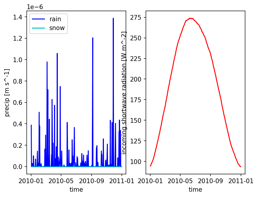
# plot one pixel as a function of time
fig = plt.figure()
ax = fig.add_subplot(121)

met_data_single_pixel = met_data_ats.isel({'time':slice(0,365),
                                           'x' : 5,
                                           'y' : 5})

met_data_single_pixel['precipitation rain [m s^-1]'].plot(color='b', label='rain')
met_data_single_pixel['precipitation snow [m SWE s^-1]'].plot(color='c', label='snow')
ax.set_ylabel('precip [m s^-1]')
ax.set_title('')
ax.legend()

ax = fig.add_subplot(122)
met_data_single_pixel['incoming shortwave radiation [W m^-2]'].plot(color='r', label='qSW_in')
ax.set_ylabel('incoming shortwave radiation [W m^-2]')
ax.set_title('')

plt.show()

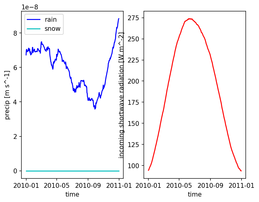
Smooth to form a typical year

A “typical” year is commonly used in a cyclic, annual steady-state spinup. We form this by averaging all Jan 1s in the record, averaging all Jan 2s, etc.

met_data

<xarray.Dataset> Size: 142MB
Dimensions:              (time: 35041, latitude: 7, longitude: 9)
Coordinates:
  * latitude             (latitude) float64 56B 35.02 35.03 ... 35.07 35.07
  * longitude            (longitude) float64 72B -83.49 -83.48 ... -83.43 -83.42
  * time                 (time) object 280kB 2010-01-01 00:00:00 ... 2013-12-...
Data variables:
    APCP_surface         (time, latitude, longitude) float64 18MB ...
    DLWRF_surface        (time, latitude, longitude) float64 18MB ...
    DSWRF_surface        (time, latitude, longitude) float64 18MB ...
    PRES_surface         (time, latitude, longitude) float64 18MB ...
    SPFH_2maboveground   (time, latitude, longitude) float64 18MB ...
    TMP_2maboveground    (time, latitude, longitude) float64 18MB ...
    UGRD_10maboveground  (time, latitude, longitude) float64 18MB ...
    VGRD_10maboveground  (time, latitude, longitude) float64 18MB ...
Attributes:
    name:     AORC v1.1
    source:   NOAA AWS S3 Zarr

xarray.Dataset

• Dimensions:
  • time: 35041
  • latitude: 7
  • longitude: 9
• Coordinates: (3)
  • latitude
    (latitude)
    float64
    35.02 35.03 35.04 ... 35.07 35.07

    long_name :

    latitude

    units :

    degrees_north

    array([35.024399, 35.032732, 35.041065, 35.049398, 35.057731, 35.066064,
           35.074397])

  • longitude
    (longitude)
    float64
    -83.49 -83.48 ... -83.43 -83.42

    long_name :

    longitude

    units :

    degrees_east

    array([-83.485194, -83.476861, -83.468528, -83.460195, -83.451862, -83.443529,
           -83.435196, -83.426863, -83.41853 ])

  • time
    (time)
    object
    2010-01-01 00:00:00 ... 2013-12-...

    array([cftime.DatetimeGregorian(2010, 1, 1, 0, 0, 0, 0, has_year_zero=False),
           cftime.DatetimeGregorian(2010, 1, 1, 1, 0, 0, 0, has_year_zero=False),
           cftime.DatetimeGregorian(2010, 1, 1, 2, 0, 0, 0, has_year_zero=False),
           ...,
           cftime.DatetimeGregorian(2013, 12, 30, 22, 0, 0, 0, has_year_zero=False),
           cftime.DatetimeGregorian(2013, 12, 30, 23, 0, 0, 0, has_year_zero=False),
           cftime.DatetimeGregorian(2013, 12, 31, 0, 0, 0, 0, has_year_zero=False)],
          shape=(35041,), dtype=object)

• Data variables: (8)
  • APCP_surface
    (time, latitude, longitude)
    float64
    ...

    AORC_Contact :

    aorc.info@noaa.gov

    aorc_version :

    v1.1

    crs :

    EPSG:4326

    level :

    surface

    long_name :

    Total Precipitation

    short_name :

    APCP_surface

    units :

    kg/m^2

    [2207583 values with dtype=float64]

  • DLWRF_surface
    (time, latitude, longitude)
    float64
    ...

    AORC_Contact :

    aorc.info@noaa.gov

    aorc_version :

    v1.1

    crs :

    EPSG:4326

    level :

    surface

    long_name :

    Downward Long-Wave Rad. Flux

    short_name :

    DLWRF_surface

    units :

    W/m^2

    [2207583 values with dtype=float64]

  • DSWRF_surface
    (time, latitude, longitude)
    float64
    ...

    AORC_Contact :

    aorc.info@noaa.gov

    aorc_version :

    v1.1

    crs :

    EPSG:4326

    level :

    surface

    long_name :

    Downward Short-Wave Rad. Flux

    short_name :

    DSWRF_surface

    units :

    W/m^2

    [2207583 values with dtype=float64]

  • PRES_surface
    (time, latitude, longitude)
    float64
    ...

    AORC_Contact :

    aorc.info@noaa.gov

    aorc_version :

    v1.1

    crs :

    EPSG:4326

    level :

    surface

    long_name :

    Pressure

    short_name :

    PRES_surface

    units :

    Pa

    [2207583 values with dtype=float64]

  • SPFH_2maboveground
    (time, latitude, longitude)
    float64
    ...

    AORC_Contact :

    aorc.info@noaa.gov

    aorc_version :

    v1.1

    crs :

    EPSG:4326

    level :

    2 m above ground

    long_name :

    Specific Humidity

    short_name :

    SPFH_2maboveground

    units :

    kg/kg

    [2207583 values with dtype=float64]

  • TMP_2maboveground
    (time, latitude, longitude)
    float64
    ...

    AORC_Contact :

    aorc.info@noaa.gov

    aorc_version :

    v1.1

    crs :

    EPSG:4326

    level :

    2 m above ground

    long_name :

    Temperature

    short_name :

    TMP_2maboveground

    units :

    K

    [2207583 values with dtype=float64]

  • UGRD_10maboveground
    (time, latitude, longitude)
    float64
    ...

    AORC_Contact :

    aorc.info@noaa.gov

    aorc_version :

    v1.1

    crs :

    EPSG:4326

    level :

    10 m above ground

    long_name :

    U-Component of Wind

    short_name :

    UGRD_10maboveground

    units :

    m/s

    [2207583 values with dtype=float64]

  • VGRD_10maboveground
    (time, latitude, longitude)
    float64
    ...

    AORC_Contact :

    aorc.info@noaa.gov

    aorc_version :

    v1.1

    crs :

    EPSG:4326

    level :

    10 m above ground

    long_name :

    V-Component of Wind

    short_name :

    VGRD_10maboveground

    units :

    m/s

    [2207583 values with dtype=float64]

• Indexes: (3)
  • latitude
    PandasIndex

    PandasIndex(Index([35.024398999999995, 35.032731999999996, 35.041064999999996,
                    35.049398,          35.057731,          35.066064,
                    35.074397],
          dtype='float64', name='latitude'))

  • longitude
    PandasIndex

    PandasIndex(Index([-83.48519400003761, -83.47686100003762, -83.46852800003762,
           -83.46019500003763, -83.45186200003764, -83.44352900003764,
           -83.43519600003765, -83.42686300003766, -83.41853000003766],
          dtype='float64', name='longitude'))

  • time
    PandasIndex

    PandasIndex(CFTimeIndex([2010-01-01 00:00:00, 2010-01-01 01:00:00, 2010-01-01 02:00:00,
                 2010-01-01 03:00:00, 2010-01-01 04:00:00, 2010-01-01 05:00:00,
                 2010-01-01 06:00:00, 2010-01-01 07:00:00, 2010-01-01 08:00:00,
                 2010-01-01 09:00:00,
                 ...
                 2013-12-30 15:00:00, 2013-12-30 16:00:00, 2013-12-30 17:00:00,
                 2013-12-30 18:00:00, 2013-12-30 19:00:00, 2013-12-30 20:00:00,
                 2013-12-30 21:00:00, 2013-12-30 22:00:00, 2013-12-30 23:00:00,
                 2013-12-31 00:00:00],
                dtype='object', length=35041, calendar='standard', freq='h'))

• Attributes: (2)

  name :

  AORC v1.1

  source :

  NOAA AWS S3 Zarr

# aggregate to daily data
met_data_daily = met_data.resample(time=datetime.timedelta(hours=24)).mean()

ndays = met_data_daily['APCP_surface'].shape[0]
print('nyears = ', ndays // 365)
print('n days leftover = ', ndays % 365)
print('note, that leftover day is a leap day')

nyears =  4
n days leftover =  1
note, that leftover day is a leap day

# cannot compute a typical year for leap year -- need to align days-of-the-year

# remove leap day (Dec 31 of leap years)
met_data_noleap = watershed_workflow.data.filterLeapDay(met_data_daily)

# smooth the raw data
met_data_smooth = watershed_workflow.data.smoothTimeSeries(met_data_noleap, method='savgol', window_length=181, polyorder=2)

# then compute a "typical" year
met_data_typical = watershed_workflow.data.computeAverageYear(met_data_smooth, 'time', 2010, 2)

# then reproject
met_data_typical_warped = watershed_workflow.warp.dataset(met_data_typical, crs, 'bilinear')

# and lastly convert to ATS
met_data_typical_ats = watershed_workflow.meteorology.convertAORCToATS(met_data_typical_warped)

# plot one pixel as a function of time
fig = plt.figure()
ax = fig.add_subplot(121)

met_data_single_pixel = met_data_typical_ats.isel({'time':slice(0,365),
                                           'x' : 5,
                                           'y' : 5})

met_data_single_pixel['precipitation rain [m s^-1]'].plot(color='b', label='rain')
met_data_single_pixel['precipitation snow [m SWE s^-1]'].plot(color='c', label='snow')
ax.set_ylabel('precip [m s^-1]')
ax.set_title('')
ax.legend()

ax = fig.add_subplot(122)
met_data_single_pixel['incoming shortwave radiation [W m^-2]'].plot(color='r', label='qSW_in')
ax.set_ylabel('incoming shortwave radiation [W m^-2]')
ax.set_title('')

plt.show()

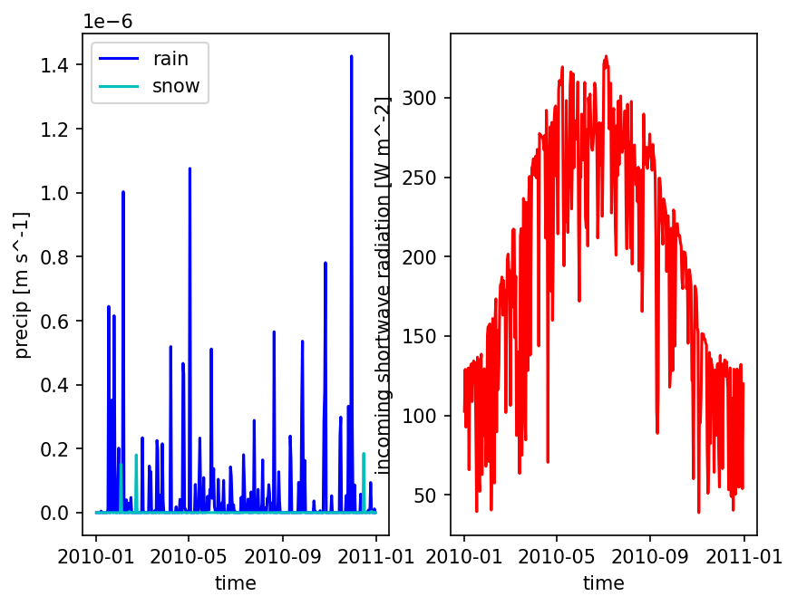
Other choices for Precip

Often smoothing precip like that is a bad idea – you now have every day misting with low intensity rain which can result in a ton of interception and canopy evaporation and no transpiration. Another approach is to just take the median total rainfall year and repeat that year multiple times.

met_data_noleap['APCP_surface'].shape[0] % 365

0

precip_raw = met_data_noleap['APCP_surface']
shape_xy = precip_raw.shape[1:]

precip_raw = precip_raw.values.reshape((-1, 365,)+shape_xy)
annual_precip_raw = precip_raw.sum(axis=(1,2,3))
print(annual_precip_raw)

[4867.39590586 5486.27508175 5143.10007664 7351.33344288]

# find the median...
# note -- don't use np.median here... for even number of years it will not appear.  Instead, sort and take the halfway point
median_i = sorted(((i,v) for (i,v) in enumerate(annual_precip_raw)), key=lambda x : x[1])[len(annual_precip_raw)//2][0]

spatially_averaged_typical_year_precip = precip_raw[median_i]
spatially_averaged_typical_year_precip.shape

(365, 7, 9)

# stuff the median year into the typical data, tiled for number of years being generated (here 2)
typical_precip_raw = np.tile(precip_raw[median_i], (2,1,1))
met_data_typical['APCP_surface'] = (['time', 'latitude', 'longitude'], typical_precip_raw)

# then reproject
met_data_typical_warped = watershed_workflow.warp.dataset(met_data_typical, crs, 'bilinear')

# convert that to ATS
met_data_typical_ats = watershed_workflow.meteorology.convertAORCToATS(met_data_typical_warped)

# plot one pixel as a function of time
fig = plt.figure()
ax = fig.add_subplot(121)

met_data_single_pixel = met_data_typical_ats.isel({'time':slice(0,365),
                                           'x' : 5,
                                           'y' : 5})

met_data_single_pixel['precipitation rain [m s^-1]'].plot(color='b', label='rain')
met_data_single_pixel['precipitation snow [m SWE s^-1]'].plot(color='c', label='snow')
ax.set_ylabel('precip [m s^-1]')
ax.set_title('')
ax.legend()

ax = fig.add_subplot(122)
met_data_single_pixel['incoming shortwave radiation [W m^-2]'].plot(color='r', label='qSW_in')
ax.set_ylabel('incoming shortwave radiation [W m^-2]')
ax.set_title('')

plt.show()