Complete Workflow for generating ATS input for Coweeta

This workflow provides a complete working example to develop a simulation campaign for integrated hydrology within ATS.

It uses the following datasets:

• NHD Plus for hydrography.

• 3DEP for elevation

• NLCD for land cover/transpiration/rooting depths

• MODIS for LAI

• GLYHMPS geology data for structural formations

• Pelletier for depth to bedrock and soil texture information

• SSURGO for soil data, where available, in the top 2m.

Given some basic inputs (in the next cell) including a NAME, this workflow creates the following files, all of which will reside in output_data:

• Mesh file: Coweeta.exo, includes all labeled sets

• Forcing: DayMet data – daily raster of precip, RH, incoming radiation, etc.

  • Coweeta_daymet_2010_2011.h5, the DayMet data on this watershed

  • Coweeta_daymet_CyclicSteadystate.h5, a “typical year” of DayMet, smoothed for spinup purposes, then looped certain number of years

• Forcing: LAI data – every 4 days, time series by land cover type of LAI.

  • Coweeta_LAI_MODIS_transient.h5, the LAI, interpolated and smoothed from the raw MODIS data

  • Coweeta_LAI_MODIS_CyclicSteadystate.h5, a “typical year” of LAI, smoothed for spinup purposes then looped 10 years

• ATS Input files for three runs, intended to be run sequentially:

  • Coweeta_steadystate.xml the steady-state solution based on uniform application of mean rainfall rate

  • Coweeta_cyclic_steadystate.xml the cyclic steady state based on typical years

  • Coweeta_transient.xml the forward model, run from 2010 – 2011

# these can be turned on for development work
%load_ext autoreload
%autoreload 2

## FIX ME -- why is this broken without importing netcdf first?
import netCDF4

# setting up logging first or else it gets preempted by another package
import watershed_workflow.ui
watershed_workflow.ui.setup_logging(1)

import os,sys
import logging
import numpy as np
from matplotlib import pyplot as plt
from matplotlib import cm as pcm
import shapely
import pandas as pd
import geopandas as gpd
import cftime, datetime
pd.options.display.max_columns = None


## provide paths to relevant packages for mesh and input file generation 
# Set paths to relevant packages for mesh and input file generation
# Update these paths to match your local installation
#
#sys.path.append('/path/to/seacas/lib')
#%set_env AMANZI_SRC_DIR=/path/to/amanzi
#%set_env ATS_SRC_DIR=/path/to/amanzi/src/physics/ats
#sys.path.append('/path/to/amanzi/tools/amanzi_xml')


import watershed_workflow 
import watershed_workflow.config
import watershed_workflow.sources
import watershed_workflow.utils
import watershed_workflow.plot
import watershed_workflow.mesh
import watershed_workflow.regions
import watershed_workflow.meteorology
import watershed_workflow.land_cover_properties
import watershed_workflow.resampling
import watershed_workflow.condition
import watershed_workflow.io
import watershed_workflow.sources.standard_names as names

import ats_input_spec
import ats_input_spec.public
import ats_input_spec.io

import amanzi_xml.utils.io as aio
import amanzi_xml.utils.search as asearch
import amanzi_xml.utils.errors as aerrors

# set the default figure size for notebooks
plt.rcParams["figure.figsize"] = (8, 6)

Input: Parameters and other source data

Note, this section will need to be modified for other runs of this workflow in other regions.

# Force Watershed Workflow to pull data from this directory rather than a shared data directory.
# This picks up the Coweeta-specific datasets set up here to avoid large file downloads for 
# demonstration purposes.
#
def splitPathFull(path):
    """
    Splits an absolute path into a list of components such that
    os.path.join(*splitPathFull(path)) == path
    """
    parts = []
    while True:
        head, tail = os.path.split(path)
        if head == path:  # root on Unix or drive letter with backslash on Windows (e.g., C:\)
            parts.insert(0, head)
            break
        elif tail == path:  # just a single file or directory
            parts.insert(0, tail)
            break
        else:
            parts.insert(0, tail)
            path = head
    return parts

cwd = splitPathFull(os.getcwd())

# REMOVE THIS PORTION OF THE CELL for general use outside of Coweeta -- this is just locating 
# the working directory within the WW directory structure
if cwd[-1] == 'Coweeta':
    pass
elif cwd[-1] == 'examples':
    cwd.append('Coweeta')
else:
    cwd.extend(['examples','Coweeta'])
# END REMOVE THIS PORTION

# Note, this directory is where downloaded data will be put as well
data_dir = os.path.join(*(cwd + ['input_data',]))
def toInput(filename):
    return os.path.join(data_dir, filename)

output_dir = os.path.join(*(cwd + ['output_data',]))
def toOutput(filename):
    return os.path.join(output_dir, filename)

work_dir = os.path.join(*cwd)
def toWorkingDir(filename):
    return os.path.join(work_dir, filename)
       

# Set the data directory to the local space to get the locally downloaded files
# REMOVE THIS CELL for general use outside fo Coweeta
watershed_workflow.config.setDataDirectory(data_dir)

## Parameters cell -- this provides all parameters that can be changed via pipelining to generate a new watershed. 
name = 'Coweeta'
coweeta_shapefile = os.path.join('input_data', 'coweeta_basin.shp')

# Geometric parameters
# -- parameters to clean and reduce the river network prior to meshing
simplify = 60                   # length scale to target average edge 
ignore_small_rivers = 2         # remove rivers with fewer than this number of reaches -- important for NHDPlus HR 
prune_by_area_fraction = 0.01   # prune any reaches whose contributing area is less than this fraction of the domain

# -- mesh triangle refinement control
refine_d0 = 200
refine_d1 = 600

#refine_L0 = 75
#refine_L1 = 200

refine_L0 = 125
refine_L1 = 300

refine_A0 = refine_L0**2 / 2
refine_A1 = refine_L1**2 / 2

# Simulation control
# - note that we use the NoLeap calendar, same as DayMet.  Simulations are typically run over the "water year"
#   which starts August 1.
start = cftime.DatetimeNoLeap(2010,8,1)
end = cftime.DatetimeNoLeap(2014,8,1)

nyears_cyclic_steadystate = 4   # how many years to run spinup

# Global Soil Properties
min_porosity = 0.05 # minimum porosity considered "too small"
max_permeability = 1.e-10 # max value considered "too permeable"
max_vg_alpha = 1.e-3 # max value of van Genuchten's alpha -- our correlation is not valid for some soils

# a dictionary of output_filenames -- will include all filenames generated
output_filenames = {}

# Note that, by default, we tend to work in the DayMet CRS because this allows us to avoid
# reprojecting meteorological forcing datasets.
crs = watershed_workflow.crs.default_crs

# get the shape and crs of the shape
coweeta_source = watershed_workflow.sources.ManagerShapefile(coweeta_shapefile)
coweeta = coweeta_source.getShapes(out_crs=crs)
coweeta.rename(columns={'AREA' : names.AREA}, inplace=True)

2025-08-29 17:27:33,176 - root - INFO: fixing column: geometry

# set up a dictionary of source objects
#
# Data sources, also called managers, deal with downloading and parsing data files from a variety of online APIs.
sources = watershed_workflow.sources.getDefaultSources()
sources['hydrography'] = watershed_workflow.sources.hydrography_sources['NHDPlus HR']

#
# This demo uses a few datasets that have been clipped out of larger, national
# datasets and are distributed with the code.  This is simply to save download
# time for this simple problem and to lower the barrier for trying out
# Watershed Workflow.  A more typical workflow would delete these lines (as 
# these files would not exist for other watersheds).
#
# The default versions of these download large raster and shapefile files that
# are defined over a very large region (globally or the entire US).
#
# DELETE THIS SECTION for non-Coweeta runs
dtb_file = os.path.join(data_dir, 'soil_structure', 'DTB', 'DTB.tif')
geo_file = os.path.join(data_dir, 'soil_structure', 'GLHYMPS', 'GLHYMPS.shp')

# GLHYMPs is a several-GB download, so we have sliced it and included the slice here
sources['geologic structure'] = watershed_workflow.sources.ManagerGLHYMPS(geo_file)

# The Pelletier DTB map is not particularly accurate at Coweeta -- the SoilGrids map seems to be better.
# Here we will use a clipped version of that map.
sources['depth to bedrock'] = watershed_workflow.sources.ManagerRaster(dtb_file)

# END DELETE THIS SECTION

# log the sources that will be used here
watershed_workflow.sources.logSources(sources)

2025-08-29 17:27:33,193 - root - INFO: Using sources:
2025-08-29 17:27:33,194 - root - INFO: --------------
2025-08-29 17:27:33,194 - root - INFO: HUC: WBD
2025-08-29 17:27:33,194 - root - INFO: hydrography: NHDPlus HR
2025-08-29 17:27:33,194 - root - INFO: DEM: 3DEP
2025-08-29 17:27:33,194 - root - INFO: soil structure: National Resources Conservation Service Soil Survey (NRCS Soils)
2025-08-29 17:27:33,195 - root - INFO: geologic structure: shapefile: "GLHYMPS.shp"
2025-08-29 17:27:33,195 - root - INFO: land cover: NLCD 2021 L48
2025-08-29 17:27:33,195 - root - INFO: LAI: MODIS
2025-08-29 17:27:33,195 - root - INFO: depth to bedrock: raster: "DTB.tif"
2025-08-29 17:27:33,195 - root - INFO: meteorology: AORC v1.1

Basin Geometry

In this section, we choose the basin, the streams to be included in the stream-aligned mesh, and make sure that all are resolved discretely at appropriate length scales for this work.

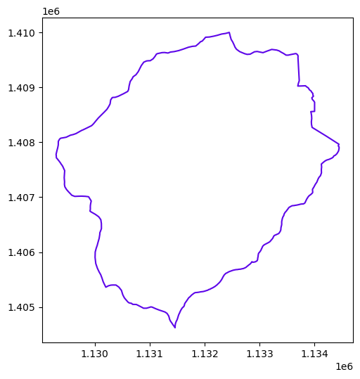
the Watershed

# Construct and plot the WW object used for storing watersheds
watershed = watershed_workflow.split_hucs.SplitHUCs(coweeta)
watershed.plot()

2025-08-29 17:27:33,207 - root - INFO: Removing holes on 1 polygons
2025-08-29 17:27:33,207 - root - INFO:   -- removed interior
2025-08-29 17:27:33,207 - root - INFO:   -- union
2025-08-29 17:27:33,208 - root - INFO: Parsing 1 components for holes
2025-08-29 17:27:33,208 - root - INFO:   -- complete

<Axes: >

the Rivers

# download/collect the river network within that shape's bounds
reaches = sources['hydrography'].getShapesByGeometry(watershed.exterior, crs, out_crs=crs)
rivers = watershed_workflow.river_tree.createRivers(reaches, method='hydroseq')

watershed_orig, rivers_orig = watershed, rivers

2025-08-29 17:27:33,369 - root - INFO: fixing column: catchment
2025-08-29 17:27:33,394 - root - INFO: fixing column: geometry

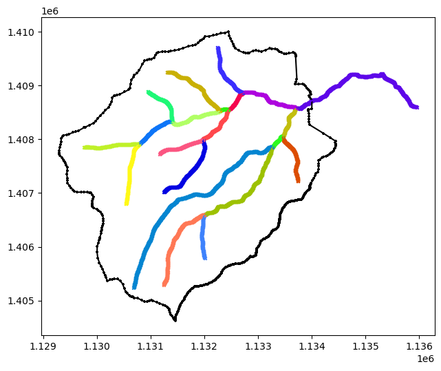
# plot the rivers and watershed
def plot(ws, rivs, ax=None):
    if ax is None:
        fig, ax = plt.subplots(1, 1)
    ws.plot(color='k', marker='+', markersize=10, ax=ax)
    for river in rivs:
        river.plot(marker='x', markersize=10, ax=ax)

plot(watershed, rivers)

# keeping the originals for plotting comparisons
def createCopy(watershed, rivers):
    """To compare before/after, we often want to create copies.  Note in real workflows most things are done in-place without copies."""
    return watershed.deepcopy(), [r.deepcopy() for r in rivers]
    

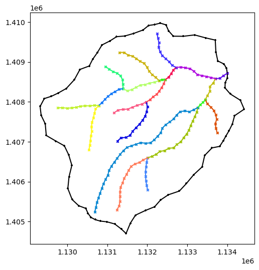
watershed, rivers = createCopy(watershed_orig, rivers_orig)

# simplifying -- this sets the discrete length scale of both the watershed boundary and the rivers
watershed_workflow.simplify(watershed, rivers, refine_L0, refine_L1, refine_d0, refine_d1)

# simplify may remove reaches from the rivers object
# -- this call removes any reaches from the dataframe as well, signaling we are all done removing reaches
#
# ETC: NOTE -- can this be moved into the simplify call?
for river in rivers:
    river.resetDataFrame()

# Now that the river network is set, find the watershed boundary outlets
for river in rivers:
    watershed_workflow.hydrography.findOutletsByCrossings(watershed, river)

2025-08-29 17:27:33,537 - root - INFO: 
2025-08-29 17:27:33,538 - root - INFO: Simplifying
2025-08-29 17:27:33,538 - root - INFO: ------------------------------
2025-08-29 17:27:33,538 - root - INFO: EPSG:5070
2025-08-29 17:27:33,538 - root - INFO: Presimplify to remove colinear, coincident points.
2025-08-29 17:27:33,541 - root - INFO: EPSG:5070
2025-08-29 17:27:33,541 - root - INFO: Pruning leaf reaches < 125
2025-08-29 17:27:33,541 - root - INFO: EPSG:5070
2025-08-29 17:27:33,541 - root - INFO: Merging internal reaches < 125
2025-08-29 17:27:33,542 - root - INFO: EPSG:5070
2025-08-29 17:27:33,543 - root - INFO:   reach: min seg length: 	    4.7213180356 	min geom length: 	  165.1231825964
2025-08-29 17:27:33,543 - root - INFO:   reach: med seg length: 	    5.7469025717 	med geom length: 	  987.4061283623
2025-08-29 17:27:33,544 - root - INFO:   reach: max seg length: 	   28.5938776319 	max geom length: 	 4068.7144554535
2025-08-29 17:27:33,544 - root - INFO: 
2025-08-29 17:27:33,544 - root - INFO:   HUC  : min seg length: 	    6.0930862643 	min geom length: 	17512.5502326232
2025-08-29 17:27:33,544 - root - INFO:   HUC  : med seg length: 	   20.1756923959 	med geom length: 	17512.5502326232
2025-08-29 17:27:33,544 - root - INFO:   HUC  : max seg length: 	  424.3827967365 	max geom length: 	17512.5502326232
2025-08-29 17:27:33,544 - root - INFO: 
2025-08-29 17:27:33,544 - root - INFO: Snapping discrete points to make rivers and HUCs discretely consistent.
2025-08-29 17:27:33,545 - root - INFO:  -- snapping HUC triple junctions to reaches
2025-08-29 17:27:33,546 - root - INFO:   reach: min seg length: 	    4.7213180356 	min geom length: 	  165.1231825964
2025-08-29 17:27:33,546 - root - INFO:   reach: med seg length: 	    5.7469025717 	med geom length: 	  987.4061283623
2025-08-29 17:27:33,546 - root - INFO:   reach: max seg length: 	   28.5938776319 	max geom length: 	 4068.7144554535
2025-08-29 17:27:33,546 - root - INFO: 
2025-08-29 17:27:33,547 - root - INFO:   HUC  : min seg length: 	    6.0930862643 	min geom length: 	17512.5502326232
2025-08-29 17:27:33,547 - root - INFO:   HUC  : med seg length: 	   20.1756923959 	med geom length: 	17512.5502326232
2025-08-29 17:27:33,547 - root - INFO:   HUC  : max seg length: 	  424.3827967365 	max geom length: 	17512.5502326232
2025-08-29 17:27:33,547 - root - INFO: 
2025-08-29 17:27:33,547 - root - INFO: EPSG:5070
2025-08-29 17:27:33,547 - root - INFO:  -- snapping reach endpoints to HUC boundaries
2025-08-29 17:27:33,555 - root - INFO:   reach: min seg length: 	    4.7213180356 	min geom length: 	  165.1231825964
2025-08-29 17:27:33,555 - root - INFO:   reach: med seg length: 	    5.7469025717 	med geom length: 	  987.4061283623
2025-08-29 17:27:33,556 - root - INFO:   reach: max seg length: 	   28.5938776319 	max geom length: 	 4068.7144554535
2025-08-29 17:27:33,556 - root - INFO: 
2025-08-29 17:27:33,556 - root - INFO:   HUC  : min seg length: 	    6.0930862643 	min geom length: 	17512.5502326232
2025-08-29 17:27:33,556 - root - INFO:   HUC  : med seg length: 	   20.1756923959 	med geom length: 	17512.5502326232
2025-08-29 17:27:33,556 - root - INFO:   HUC  : max seg length: 	  424.3827967365 	max geom length: 	17512.5502326232
2025-08-29 17:27:33,556 - root - INFO: 
2025-08-29 17:27:33,557 - root - INFO: EPSG:5070
2025-08-29 17:27:33,557 - root - INFO:  -- cutting reaches at HUC boundaries
2025-08-29 17:27:33,557 - root - INFO: intersection found
2025-08-29 17:27:33,557 - root - INFO:   - cutting reach at external boundary of HUCs:
2025-08-29 17:27:33,558 - root - INFO:       split HUC boundary ls into 2 pieces
2025-08-29 17:27:33,558 - root - INFO:       split reach ls into 2 pieces
2025-08-29 17:27:33,560 - root - INFO:   reach: min seg length: 	    2.0814263569 	min geom length: 	  165.1231825964
2025-08-29 17:27:33,560 - root - INFO:   reach: med seg length: 	    5.7506498560 	med geom length: 	  944.9293512284
2025-08-29 17:27:33,561 - root - INFO:   reach: max seg length: 	   28.5938776319 	max geom length: 	 4068.7144554535
2025-08-29 17:27:33,561 - root - INFO: 
2025-08-29 17:27:33,562 - root - INFO:   HUC  : min seg length: 	    6.0930862643 	min geom length: 	 4627.5195485168
2025-08-29 17:27:33,562 - root - INFO:   HUC  : med seg length: 	   20.1371178909 	med geom length: 	 8756.2751163116
2025-08-29 17:27:33,562 - root - INFO:   HUC  : max seg length: 	  424.3827967365 	max geom length: 	12885.0306841065
2025-08-29 17:27:33,562 - root - INFO: 
2025-08-29 17:27:33,563 - root - INFO: EPSG:5070
2025-08-29 17:27:33,563 - root - INFO: 
2025-08-29 17:27:33,563 - root - INFO: Simplification Diagnostics
2025-08-29 17:27:33,564 - root - INFO: ------------------------------
2025-08-29 17:27:33,564 - root - INFO:   reach: min seg length: 	    2.0814263569 	min geom length: 	  165.1231825964
2025-08-29 17:27:33,564 - root - INFO:   reach: med seg length: 	    5.7506498560 	med geom length: 	  944.9293512284
2025-08-29 17:27:33,564 - root - INFO:   reach: max seg length: 	   28.5938776319 	max geom length: 	 4068.7144554535
2025-08-29 17:27:33,565 - root - INFO: 
2025-08-29 17:27:33,565 - root - INFO:   HUC  : min seg length: 	    6.0930862643 	min geom length: 	 4627.5195485168
2025-08-29 17:27:33,565 - root - INFO:   HUC  : med seg length: 	   20.1371178909 	med geom length: 	 8756.2751163116
2025-08-29 17:27:33,565 - root - INFO:   HUC  : max seg length: 	  424.3827967365 	max geom length: 	12885.0306841065
2025-08-29 17:27:33,565 - root - INFO: 
2025-08-29 17:27:33,565 - root - INFO: EPSG:5070
2025-08-29 17:27:33,566 - root - INFO: 
2025-08-29 17:27:33,566 - root - INFO: Resampling HUC and river
2025-08-29 17:27:33,566 - root - INFO: ------------------------------
2025-08-29 17:27:33,566 - root - INFO:  -- resampling HUCs based on distance function (200, 125, 600, 300)
2025-08-29 17:27:33,632 - root - INFO: EPSG:5070
2025-08-29 17:27:33,632 - root - INFO:  -- resampling reaches based on uniform target 125
2025-08-29 17:27:33,638 - root - INFO: EPSG:5070
2025-08-29 17:27:33,638 - root - INFO: 
2025-08-29 17:27:33,638 - root - INFO: Resampling Diagnostics
2025-08-29 17:27:33,638 - root - INFO: ------------------------------
2025-08-29 17:27:33,639 - root - INFO:   reach: min seg length: 	   80.6788358181 	min geom length: 	  162.6365417198
2025-08-29 17:27:33,639 - root - INFO:   reach: med seg length: 	  116.9716913444 	med geom length: 	  933.8039522688
2025-08-29 17:27:33,639 - root - INFO:   reach: max seg length: 	  124.2213863088 	max geom length: 	 4016.8050558108
2025-08-29 17:27:33,639 - root - INFO: 
2025-08-29 17:27:33,639 - root - INFO:   HUC  : min seg length: 	  123.6155631726 	min geom length: 	 4318.0632729232
2025-08-29 17:27:33,640 - root - INFO:   HUC  : med seg length: 	  225.3314175350 	med geom length: 	 8192.0964914255
2025-08-29 17:27:33,640 - root - INFO:   HUC  : max seg length: 	  299.1244344516 	max geom length: 	12066.1297099279
2025-08-29 17:27:33,640 - root - INFO: 
2025-08-29 17:27:33,640 - root - INFO: EPSG:5070
2025-08-29 17:27:33,640 - root - INFO: 
2025-08-29 17:27:33,640 - root - INFO: Clean up sharp angles, both internally and at junctions.
2025-08-29 17:27:33,641 - root - INFO: ------------------------------
2025-08-29 17:27:33,642 - root - INFO: SSA1: EPSG:5070
2025-08-29 17:27:33,644 - root - INFO: SSA2: EPSG:5070
2025-08-29 17:27:33,647 - root - INFO: SSA3: EPSG:5070
2025-08-29 17:27:33,658 - root - INFO: SSA4: EPSG:5070
2025-08-29 17:27:33,658 - root - INFO: Cleaned up 0 sharp angles.
2025-08-29 17:27:33,659 - root - INFO:   reach: min seg length: 	   80.6788358181 	min geom length: 	  162.6365417198
2025-08-29 17:27:33,659 - root - INFO:   reach: med seg length: 	  116.9716913444 	med geom length: 	  933.8039522688
2025-08-29 17:27:33,659 - root - INFO:   reach: max seg length: 	  124.2213863088 	max geom length: 	 4016.8050558108
2025-08-29 17:27:33,659 - root - INFO: 
2025-08-29 17:27:33,660 - root - INFO:   HUC  : min seg length: 	  123.6155631726 	min geom length: 	 4318.0632729232
2025-08-29 17:27:33,660 - root - INFO:   HUC  : med seg length: 	  225.3314175350 	med geom length: 	 8192.0964914255
2025-08-29 17:27:33,660 - root - INFO:   HUC  : max seg length: 	  299.1244344516 	max geom length: 	12066.1297099279
2025-08-29 17:27:33,660 - root - INFO: 
2025-08-29 17:27:33,660 - root - INFO: EPSG:5070
2025-08-29 17:27:33,671 - root - INFO: Crossings by Polygon:
2025-08-29 17:27:33,672 - root - INFO:   Polygon 0
2025-08-29 17:27:33,672 - root - INFO:     crossing: [1134002.89761532 1408719.29292113]
2025-08-29 17:27:33,672 - root - INFO: Constructing outlet list
2025-08-29 17:27:33,672 - root - INFO: Iteration = 0
2025-08-29 17:27:33,672 - root - INFO: -----------------
2025-08-29 17:27:33,673 - root - INFO:  poly outlet 0 : 0, [1134002.89761532 1408719.29292113]
2025-08-29 17:27:33,673 - root - INFO: last outlet is 0 in polygon 0 at {crossings_clusters_centroids[last_outlet]}

plot(watershed, rivers)

# this generates a zoomable map, showing different reaches and watersheds, 
# with discrete points.  Problem areas are clickable to get IDs for manual
# modifications.
m = watershed.explore(marker=False)
for river in rivers_orig:
    m = river.explore(m=m, column=None, color='black', name=river['name']+' raw', marker=False)
for river in rivers:
    m = river.explore(m=m)
    
m = watershed_workflow.makeMap(m)
m

Make this Notebook Trusted to load map: File -> Trust Notebook

Mesh Geometry

Discretely create the stream-aligned mesh. Download elevation data, and condition the mesh discretely to make for better topography.

# Refine triangles if they get too acute
min_angle = 32 # degrees

# width of reach by stream order (order:width)
widths = dict({1:8,2:12,3:16})

# create the mesh
m2, areas, dists = watershed_workflow.tessalateRiverAligned(watershed, rivers, 
                                                            river_width=widths,
                                                            refine_min_angle=min_angle,
                                                            refine_distance=[refine_d0, refine_A0, refine_d1, refine_A1],
                                                            diagnostics=True)

2025-08-29 17:27:33,945 - root - INFO: 
2025-08-29 17:27:33,946 - root - INFO: Stream-aligned Meshing
2025-08-29 17:27:33,946 - root - INFO: ------------------------------
2025-08-29 17:27:33,946 - root - INFO: Creating stream-aligned mesh...
2025-08-29 17:27:33,965 - root - INFO: Adjusting HUC to match reaches at outlet
2025-08-29 17:27:33,973 - root - INFO: 
2025-08-29 17:27:33,974 - root - INFO: Triangulation
2025-08-29 17:27:33,974 - root - INFO: ------------------------------
2025-08-29 17:27:33,978 - root - INFO: Triangulating...
2025-08-29 17:27:33,979 - root - INFO:    455 points and 456 facets
2025-08-29 17:27:33,979 - root - INFO:  checking graph consistency
2025-08-29 17:27:33,979 - root - INFO:  tolerance is set to 1.0
2025-08-29 17:27:33,981 - root - INFO:  building graph data structures
2025-08-29 17:27:33,982 - root - INFO:  triangle.build...
2025-08-29 17:27:34,114 - root - INFO:   ...built: 1475 mesh points and 2493 triangles
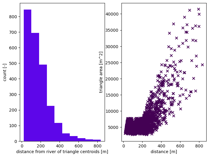
2025-08-29 17:27:34,115 - root - INFO: Plotting triangulation diagnostics
2025-08-29 17:27:34,162 - root - INFO:   min area = 2656.7518310546875
2025-08-29 17:27:34,162 - root - INFO:   max area = 41455.08837890625

# get a raster for the elevation map, based on 3DEP
dem = sources['DEM'].getDataset(watershed.exterior.buffer(100), watershed.crs)['dem']

# provide surface mesh elevations
watershed_workflow.elevate(m2, dem)

2025-08-29 17:27:34,313 - root - INFO: Incoming shape area = 0.0017688403168597767
2025-08-29 17:27:34,313 - root - INFO: ... buffering incoming shape by = 0.00108
2025-08-29 17:27:34,314 - root - INFO: ... buffered shape area = 0.001956767422135052
2025-08-29 17:27:34,314 - root - INFO: Getting DEM with map of area = 0.001956767422135052

# Plot the DEM raster
fig, ax = plt.subplots()

# Plot the DEM data
im = dem.plot(ax=ax, cmap='terrain', add_colorbar=False)

# Add colorbar
cbar = plt.colorbar(im, ax=ax, shrink=0.8)
cbar.set_label('Elevation (m)', rotation=270, labelpad=15)

# Add title and labels
ax.set_title('Digital Elevation Model (DEM)', fontsize=14, fontweight='bold')
ax.set_xlabel('X Coordinate')
ax.set_ylabel('Y Coordinate')

# Set equal aspect ratio
ax.set_aspect('equal')

plt.tight_layout()
plt.show()

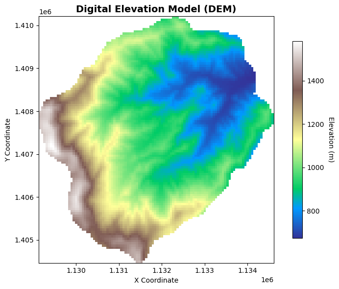
In the pit-filling algorithm, we want to make sure that river corridor is not filled up. Hence we exclude river corridor cells from the pit-filling algorithm.

# hydrologically condition the mesh, removing pits
river_mask=np.zeros((len(m2.conn)))
for i, elem in enumerate(m2.conn):
    if not len(elem)==3:
        river_mask[i]=1     
watershed_workflow.condition.fillPitsDual(m2, is_waterbody=river_mask)

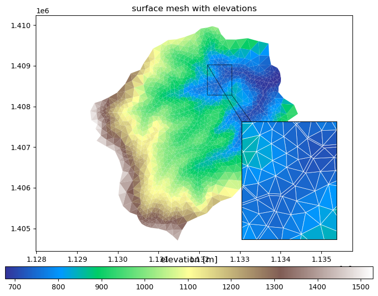
There are a range of options to condition river corridor mesh. We hydrologically condition the river mesh, ensuring unimpeded water flow in river corridors by globally adjusting flowlines to rectify artificial obstructions from inconsistent DEM elevations or misalignments. Please read the documentation for more information

# conditioning river mesh
#
# adding elevations to the river tree for stream bed conditioning
watershed_workflow.condition.setProfileByDEM(rivers, dem)

# conditioning the river mesh using NHD elevations
watershed_workflow.condition.conditionRiverMesh(m2, rivers[0])

# plotting surface mesh with elevations
fig, ax = plt.subplots()
ax2 = ax.inset_axes([0.65,0.05,0.3,0.5])
cbax = fig.add_axes([0.05,0.02,0.9,0.04])

mp = m2.plot(facecolors='elevation', edgecolors=None, ax=ax, linewidth=0.5, colorbar=False)
cbar = fig.colorbar(mp, orientation="horizontal", cax=cbax)
ax.set_title('surface mesh with elevations')
ax.set_aspect('equal', 'datalim')

mp2 = m2.plot(facecolors='elevation', edgecolors='white', ax=ax2, colorbar=False)
ax2.set_aspect('equal', 'datalim')

xlim = (1.1322e6, 1.1328e6)
ylim = (1.4085e6, 1.4088e6)

ax2.set_xlim(xlim)
ax2.set_ylim(ylim)
ax2.set_xticks([])
ax2.set_yticks([])

ax.indicate_inset_zoom(ax2, edgecolor='k')

cbar.ax.set_title('elevation [m]')

plt.show()

2025-08-29 17:27:50,483 - matplotlib.axes._base - WARNING: Ignoring fixed y limits to fulfill fixed data aspect with adjustable data limits.

# add labeled sets for subcatchments and outlets
watershed_workflow.regions.addWatershedAndOutletRegions(m2, watershed, outlet_width=250, exterior_outlet=True)

# add labeled sets for river corridor cells
watershed_workflow.regions.addRiverCorridorRegions(m2, rivers)

# add labeled sets for river corridor cells by order
watershed_workflow.regions.addStreamOrderRegions(m2, rivers)

2025-08-29 17:27:50,586 - root - INFO: Adding regions for 1 polygons

for ls in m2.labeled_sets:
    print(f'{ls.setid} : {ls.entity} : {len(ls.ent_ids)} : "{ls.name}"')

10000 : CELL : 2683 : "0"
10001 : CELL : 2683 : "0 surface"
10002 : FACE : 76 : "0 boundary"
10003 : FACE : 5 : "0 outlet"
10004 : FACE : 5 : "surface domain outlet"
10005 : CELL : 190 : "river corridor 0 surface"
10006 : CELL : 16 : "stream order 3"
10007 : CELL : 48 : "stream order 2"
10008 : CELL : 126 : "stream order 1"

Surface properties

Meshes interact with data to provide forcing, parameters, and more in the actual simulation. Specifically, we need vegetation type on the surface to provide information about transpiration and subsurface structure to provide information about water retention curves, etc.

NLCD for LULC

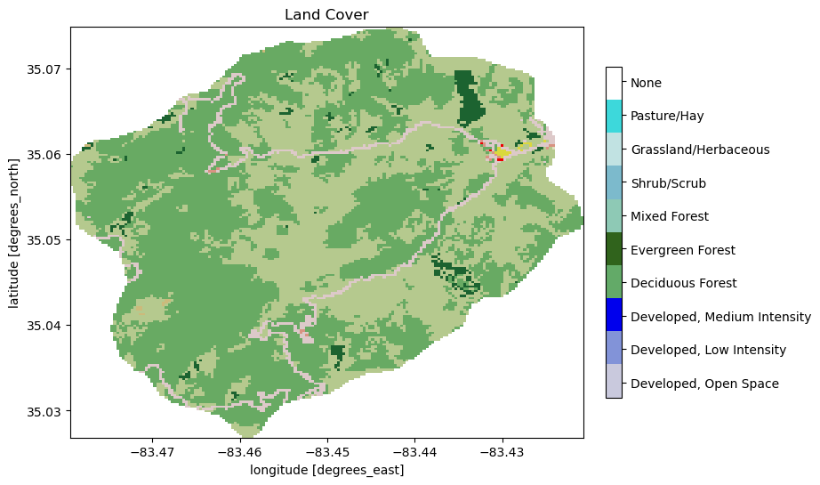
We’ll start by downloading and collecting land cover from the NLCD dataset, and generate sets for each land cover type that cover the surface. Likely these will be some combination of grass, deciduous forest, coniferous forest, and mixed.

# download the NLCD raster
nlcd = sources['land cover'].getDataset(watershed.exterior.buffer(100), watershed.crs)['cover']

# what land cover types did we get?
logging.info('Found land cover dtypes: {}'.format(nlcd.dtype))
logging.info('Found land cover types: {}'.format(set(list(nlcd.values.ravel()))))

2025-08-29 17:27:50,657 - root - INFO: Incoming shape area = 0.0017688403168597767
2025-08-29 17:27:50,657 - root - INFO: ... buffering incoming shape by = 0.00027
2025-08-29 17:27:50,657 - root - INFO: ... buffered shape area = 0.0018151848254589866
2025-08-29 17:27:50,700 - root - INFO: Found land cover dtypes: uint8
2025-08-29 17:27:50,701 - root - INFO: Found land cover types: {np.uint8(71), np.uint8(41), np.uint8(42), np.uint8(43), np.uint8(81), np.uint8(52), np.uint8(21), np.uint8(22), np.uint8(23), np.uint8(127)}

# create a colormap for the data
nlcd_indices, nlcd_cmap, nlcd_norm, nlcd_ticks, nlcd_labels = \
      watershed_workflow.colors.createNLCDColormap(np.unique(nlcd))
nlcd_cmap

making colormap with: [np.uint8(21), np.uint8(22), np.uint8(23), np.uint8(41), np.uint8(42), np.uint8(43), np.uint8(52), np.uint8(71), np.uint8(81), np.uint8(127)]
making colormap with colors: [(0.86666666667, 0.78823529412, 0.78823529412), (0.84705882353, 0.57647058824, 0.50980392157), (0.92941176471, 0.0, 0.0), (0.40784313726, 0.66666666667, 0.38823529412), (0.10980392157, 0.38823529412, 0.18823529412), (0.70980392157, 0.78823529412, 0.5568627451), (0.8, 0.72941176471, 0.4862745098), (0.8862745098, 0.8862745098, 0.7568627451), (0.85882352941, 0.84705882353, 0.23921568628), (1.0, 1.0, 1.0)]

from_list

under

bad

over

fig, ax = plt.subplots(1,1)
nlcd.plot.imshow(ax=ax, cmap=nlcd_cmap, norm=nlcd_norm, add_colorbar=False)
watershed_workflow.colors.createIndexedColorbar(ncolors=len(nlcd_indices), 
                               cmap=nlcd_cmap, labels=nlcd_labels, ax=ax) 
ax.set_title('Land Cover')
plt.show()

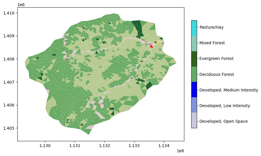
# map nlcd onto the mesh
m2_nlcd = watershed_workflow.getDatasetOnMesh(m2, nlcd, method='nearest')
m2.cell_data = pd.DataFrame({'land_cover': m2_nlcd})

# double-check that nan not in the values
assert 127 not in m2_nlcd

# create a new set of labels and indices with only those that actually appear on the mesh
nlcd_indices, nlcd_cmap, nlcd_norm, nlcd_ticks, nlcd_labels = \
      watershed_workflow.colors.createNLCDColormap(np.unique(m2_nlcd))

making colormap with: [np.uint8(21), np.uint8(22), np.uint8(23), np.uint8(41), np.uint8(42), np.uint8(43), np.uint8(81)]
making colormap with colors: [(0.86666666667, 0.78823529412, 0.78823529412), (0.84705882353, 0.57647058824, 0.50980392157), (0.92941176471, 0.0, 0.0), (0.40784313726, 0.66666666667, 0.38823529412), (0.10980392157, 0.38823529412, 0.18823529412), (0.70980392157, 0.78823529412, 0.5568627451), (0.85882352941, 0.84705882353, 0.23921568628)]

mp = m2.plot(facecolors=m2_nlcd, cmap=nlcd_cmap, norm=nlcd_norm, edgecolors=None, colorbar=False)
watershed_workflow.colors.createIndexedColorbar(ncolors=len(nlcd_indices), 
                               cmap=nlcd_cmap, labels=nlcd_labels, ax=plt.gca()) 
plt.show()

# add labeled sets to the mesh for NLCD
nlcd_labels_dict = dict(zip(nlcd_indices, nlcd_labels))
watershed_workflow.regions.addSurfaceRegions(m2, names=nlcd_labels_dict)

nlcd_labels_dict

{np.uint8(21): 'Developed, Open Space',
 np.uint8(22): 'Developed, Low Intensity',
 np.uint8(23): 'Developed, Medium Intensity',
 np.uint8(41): 'Deciduous Forest',
 np.uint8(42): 'Evergreen Forest',
 np.uint8(43): 'Mixed Forest',
 np.uint8(81): 'Pasture/Hay'}

for ls in m2.labeled_sets:
    print(f'{ls.setid} : {ls.entity} : {len(ls.ent_ids)} : "{ls.name}"')

10000 : CELL : 2683 : "0"
10001 : CELL : 2683 : "0 surface"
10002 : FACE : 76 : "0 boundary"
10003 : FACE : 5 : "0 outlet"
10004 : FACE : 5 : "surface domain outlet"
10005 : CELL : 190 : "river corridor 0 surface"
10006 : CELL : 16 : "stream order 3"
10007 : CELL : 48 : "stream order 2"
10008 : CELL : 126 : "stream order 1"
21 : CELL : 104 : "Developed, Open Space"
22 : CELL : 5 : "Developed, Low Intensity"
23 : CELL : 1 : "Developed, Medium Intensity"
41 : CELL : 1393 : "Deciduous Forest"
42 : CELL : 43 : "Evergreen Forest"
43 : CELL : 1133 : "Mixed Forest"
81 : CELL : 4 : "Pasture/Hay"

MODIS LAI

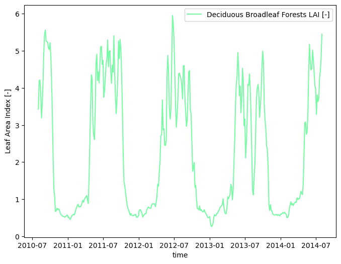
Leaf area index is needed on each land cover type – this is used in the Evapotranspiration calculation.

# download LAI and corresponding LULC datasets -- these are actually already downloaded, 
# as the MODIS AppEEARS API is quite slow
#
# Note that MODIS does NOT work with the noleap calendar, so we have to convert to actual dates first
start_leap = cftime.DatetimeGregorian(start.year, start.month, start.day)
end_leap = cftime.DatetimeGregorian(end.year, end.month, end.day)
res = sources['LAI'].getDataset(watershed.exterior, crs, start_leap, end_leap)

2025-08-29 17:27:51,060 - root - INFO: Incoming shape area = 0.0016040440731829
2025-08-29 17:27:51,061 - root - INFO: ... buffering incoming shape by = 0.0045000000000000005
2025-08-29 17:27:51,061 - root - INFO: ... buffered shape area = 0.0024043957079133795
2025-08-29 17:27:51,062 - root - INFO: Building request for bounds: [np.float64(-83.4825), np.float64(35.0235), np.float64(-83.4176), np.float64(35.0782)]
2025-08-29 17:27:51,062 - root - INFO: ... requires files:
2025-08-29 17:27:51,063 - root - INFO:  ... /home/ecoon/code/watershed_workflow/repos/master/examples/Coweeta/input_data/land_cover/MODIS/modis_LAI_08-01-2010_08-01-2014_35.0782x-83.4825_35.0235x-83.4176.nc
2025-08-29 17:27:51,063 - root - INFO:  ... /home/ecoon/code/watershed_workflow/repos/master/examples/Coweeta/input_data/land_cover/MODIS/modis_LULC_08-01-2010_08-01-2014_35.0782x-83.4825_35.0235x-83.4176.nc
2025-08-29 17:27:51,064 - root - INFO: ... files exist locally.

modis_data = res
assert modis_data['LAI'].rio.crs is not None
print(modis_data['LULC'].rio.crs, modis_data['LULC'].dtype)

EPSG:4269 float64

# MODIS data comes with time-dependent LAI AND time-dependent LULC -- just take the mode to find the most common LULC
modis_data['LULC'] = watershed_workflow.data.computeMode(modis_data['LULC'], 'time_LULC')

# now it is safe to have only one time
modis_data = modis_data.rename({'time_LAI':'time'})

# remove leap day (366th day of any leap year) to match our Noleap Calendar
modis_data = watershed_workflow.data.filterLeapDay(modis_data)

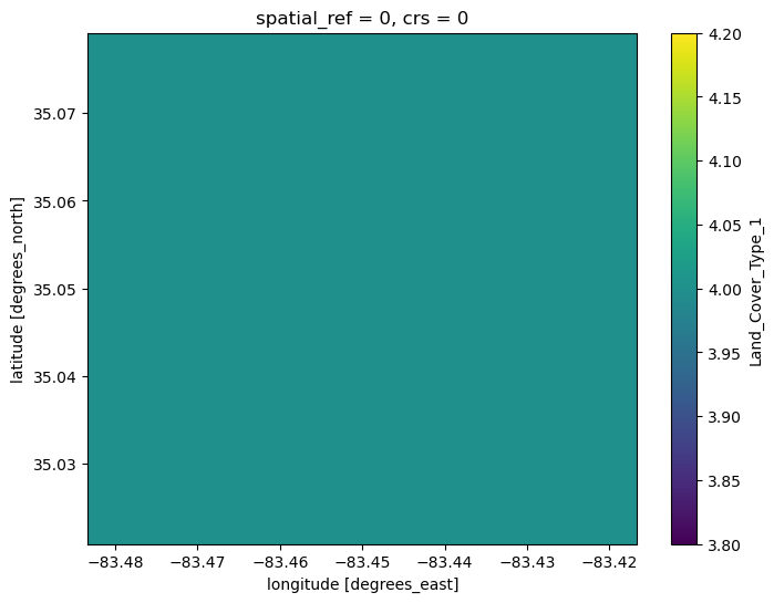
# plot the MODIS data -- note the entire domain is covered with one type for Coweeta (it is small!)
modis_data['LULC'].plot.imshow()

<matplotlib.image.AxesImage at 0x7fad5074a990>

# compute the transient time series
modis_lai = watershed_workflow.land_cover_properties.computeTimeSeries(modis_data['LAI'], modis_data['LULC'], 
                                                                      polygon=watershed.exterior, polygon_crs=watershed.crs)

modis_lai

	time	Deciduous Broadleaf Forests LAI [-]
0	2010-08-01 00:00:00	3.244086
1	2010-08-05 00:00:00	4.813978
2	2010-08-09 00:00:00	3.469892
3	2010-08-13 00:00:00	4.234409
4	2010-08-17 00:00:00	3.178495
...	...	...
364	2014-07-16 00:00:00	5.615054
365	2014-07-20 00:00:00	4.093548
366	2014-07-24 00:00:00	4.000000
367	2014-07-28 00:00:00	4.853763
368	2014-08-01 00:00:00	5.529032

369 rows × 2 columns

# smooth the data in time
modis_lai_smoothed = watershed_workflow.data.smoothTimeSeries(modis_lai, 'time')

# save the MODIS time series to disk
output_filenames['modis_lai_transient'] = toOutput(f'{name}_LAI_MODIS_transient.h5')
watershed_workflow.io.writeTimeseriesToHDF5(output_filenames['modis_lai_transient'], modis_lai_smoothed)
watershed_workflow.land_cover_properties.plotLAI(modis_lai_smoothed, indices='MODIS')

2025-08-29 17:27:51,314 - root - INFO: Writing HDF5 file: /home/ecoon/code/watershed_workflow/repos/master/examples/Coweeta/output_data/Coweeta_LAI_MODIS_transient.h5

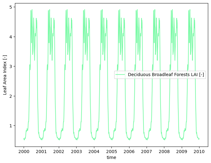
# compute a typical year
modis_lai_typical = watershed_workflow.data.computeAverageYear(modis_lai_smoothed, 'time', output_nyears=10, 
                                                                  start_year=2000)

output_filenames['modis_lai_cyclic_steadystate'] = toOutput(f'{name}_LAI_MODIS_CyclicSteadystate.h5')
watershed_workflow.io.writeTimeseriesToHDF5(output_filenames['modis_lai_cyclic_steadystate'], modis_lai_typical)
watershed_workflow.land_cover_properties.plotLAI(modis_lai_typical, indices='MODIS')

2025-08-29 17:27:51,424 - root - INFO: Writing HDF5 file: /home/ecoon/code/watershed_workflow/repos/master/examples/Coweeta/output_data/Coweeta_LAI_MODIS_CyclicSteadystate.h5

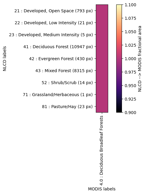
Crosswalk of LAI to NLCD LC

crosswalk = watershed_workflow.land_cover_properties.computeCrosswalk(modis_data['LULC'], nlcd, method='fractional area')

2025-08-29 17:27:51,523 - root - INFO: Compute the crosswalk between MODIS and NLCD:
2025-08-29 17:27:51,523 - root - INFO:   unique MODIS: [np.float64(4.0)]
2025-08-29 17:27:51,524 - root - INFO:   unique NLCD: [np.uint8(21), np.uint8(22), np.uint8(23), np.uint8(41), np.uint8(42), np.uint8(43), np.uint8(52), np.uint8(71), np.uint8(81)]

# Compute the NLCD-based time series
nlcd_lai_cyclic_steadystate = watershed_workflow.land_cover_properties.applyCrosswalk(crosswalk, modis_lai_typical)
nlcd_lai_transient = watershed_workflow.land_cover_properties.applyCrosswalk(crosswalk, modis_lai_smoothed)

watershed_workflow.land_cover_properties.removeNullLAI(nlcd_lai_cyclic_steadystate)
watershed_workflow.land_cover_properties.removeNullLAI(nlcd_lai_transient)
nlcd_lai_transient

None LAI [-] False
Open Water LAI [-] False
Perrenial Ice/Snow LAI [-] False
Developed, Medium Intensity LAI [-] True
Developed, High Intensity LAI [-] False
Barren Land LAI [-] False
None LAI [-] False
Open Water LAI [-] False
Perrenial Ice/Snow LAI [-] False
Developed, Medium Intensity LAI [-] True
Developed, High Intensity LAI [-] False
Barren Land LAI [-] False

	time	Developed, Open Space LAI [-]	Developed, Low Intensity LAI [-]	Developed, Medium Intensity LAI [-]	Deciduous Forest LAI [-]	Evergreen Forest LAI [-]	Mixed Forest LAI [-]	Shrub/Scrub LAI [-]	Grassland/Herbaceous LAI [-]	Pasture/Hay LAI [-]
0	2010-08-01 00:00:00	3.427880	3.427880	0.0	3.427880	3.427880	3.427880	3.427880	3.427880	3.427880
1	2010-08-05 00:00:00	4.186508	4.186508	0.0	4.186508	4.186508	4.186508	4.186508	4.186508	4.186508
2	2010-08-09 00:00:00	4.217460	4.217460	0.0	4.217460	4.217460	4.217460	4.217460	4.217460	4.217460
3	2010-08-13 00:00:00	3.842960	3.842960	0.0	3.842960	3.842960	3.842960	3.842960	3.842960	3.842960
4	2010-08-17 00:00:00	3.192524	3.192524	0.0	3.192524	3.192524	3.192524	3.192524	3.192524	3.192524
...	...	...	...	...	...	...	...	...	...	...
364	2014-07-16 00:00:00	3.712084	3.712084	0.0	3.712084	3.712084	3.712084	3.712084	3.712084	3.712084
365	2014-07-20 00:00:00	4.249360	4.249360	0.0	4.249360	4.249360	4.249360	4.249360	4.249360	4.249360
366	2014-07-24 00:00:00	4.460855	4.460855	0.0	4.460855	4.460855	4.460855	4.460855	4.460855	4.460855
367	2014-07-28 00:00:00	4.805709	4.805709	0.0	4.805709	4.805709	4.805709	4.805709	4.805709	4.805709
368	2014-08-01 00:00:00	5.453098	5.453098	0.0	5.453098	5.453098	5.453098	5.453098	5.453098	5.453098

369 rows × 10 columns

# write the NLCD-based time series to disk
output_filenames['nlcd_lai_cyclic_steadystate'] = toOutput(f'{name}_LAI_NLCD_CyclicSteadystate.h5')
watershed_workflow.io.writeTimeseriesToHDF5(output_filenames['nlcd_lai_cyclic_steadystate'], nlcd_lai_cyclic_steadystate)

output_filenames['nlcd_lai_transient'] = toOutput(f'{name}_LAI_NLCD_{start.year}_{end.year}.h5')
watershed_workflow.io.writeTimeseriesToHDF5(output_filenames['nlcd_lai_transient'], nlcd_lai_transient)

2025-08-29 17:27:51,625 - root - INFO: Writing HDF5 file: /home/ecoon/code/watershed_workflow/repos/master/examples/Coweeta/output_data/Coweeta_LAI_NLCD_CyclicSteadystate.h5
2025-08-29 17:27:51,629 - root - INFO: Writing HDF5 file: /home/ecoon/code/watershed_workflow/repos/master/examples/Coweeta/output_data/Coweeta_LAI_NLCD_2010_2014.h5

Subsurface Soil, Geologic Structure

NRCS Soils

# get NRCS shapes, on a reasonable crs
nrcs = sources['soil structure'].getShapesByGeometry(watershed.exterior, watershed.crs, out_crs=crs)
nrcs

2025-08-29 17:27:51,666 - root - INFO: Attempting to download source for target '/home/ecoon/code/watershed_workflow/repos/master/examples/Coweeta/input_data/soil_structure/SSURGO/SSURGO_-83.4780_35.0280_-83.4221_35.0737.shp'
2025-08-29 17:27:51,671 - root - INFO:   Found 456 shapes.
2025-08-29 17:27:51,722 - root - INFO: found 41 unique MUKEYs.
2025-08-29 17:27:52,049 - root - INFO: Running Rosetta for van Genutchen parameters
2025-08-29 17:27:52,086 - root - INFO:   ... done
2025-08-29 17:27:52,087 - root - INFO:   requested 41 values
2025-08-29 17:27:52,087 - root - INFO:   got 41 responses
2025-08-29 17:27:52,092 - root - INFO: fixing column: geometry

	mukey	geometry	residual saturation [-]	Rosetta porosity [-]	van Genuchten alpha [Pa^-1]	van Genuchten n [-]	Rosetta permeability [m^2]	thickness [m]	permeability [m^2]	porosity [-]	bulk density [g/cm^3]	total sand pct [%]	total silt pct [%]	total clay pct [%]	source	ID	name
0	545800	MULTIPOLYGON (((1131335.296 1404750.906, 11313...	0.177165	0.431041	0.000139	1.470755	8.079687e-13	2.03	3.429028e-15	0.307246	1.297356	66.356250	19.518750	14.125000	NRCS	545800	NRCS-545800
1	545801	MULTIPOLYGON (((1129506.994 1406944.207, 11294...	0.177493	0.432741	0.000139	1.469513	8.184952e-13	2.03	3.247236e-15	0.303714	1.292308	66.400000	19.300000	14.300000	NRCS	545801	NRCS-545801
2	545803	MULTIPOLYGON (((1130760.995 1408224.107, 11307...	0.172412	0.400889	0.000150	1.491087	6.477202e-13	2.03	2.800000e-12	0.379163	1.400000	66.799507	21.700493	11.500000	NRCS	545803	NRCS-545803
3	545805	MULTIPOLYGON (((1134255.698 1405132.204, 11342...	0.177122	0.388687	0.000083	1.468789	3.412748e-13	2.03	2.800000e-12	0.384877	1.400000	46.721675	41.778325	11.500000	NRCS	545805	NRCS-545805
4	545806	MULTIPOLYGON (((1134180.798 1405169.304, 11341...	0.177122	0.388687	0.000083	1.468789	3.412748e-13	2.03	2.800000e-12	0.384877	1.400000	46.721675	41.778325	11.500000	NRCS	545806	NRCS-545806
5	545807	MULTIPOLYGON (((1131255.496 1405664.406, 11312...	0.177122	0.388687	0.000083	1.468789	3.412748e-13	2.03	2.800000e-12	0.384877	1.400000	46.721675	41.778325	11.500000	NRCS	545807	NRCS-545807
6	545811	MULTIPOLYGON (((1130078.796 1404597.506, 11300...	0.185628	0.387114	0.000166	1.473045	4.803887e-13	2.03	1.830706e-12	0.329821	1.488889	69.043320	17.115010	13.841670	NRCS	545811	NRCS-545811
7	545812	POLYGON ((1130078.496 1404548.906, 1130061.396...	0.185628	0.387114	0.000166	1.473045	4.803887e-13	2.03	1.830706e-12	0.329821	1.488889	69.043320	17.115010	13.841670	NRCS	545812	NRCS-545812
8	545813	MULTIPOLYGON (((1132919.997 1405040.305, 11329...	0.183468	0.398767	0.000127	1.445858	4.296896e-13	2.03	6.219065e-14	0.349442	1.410667	60.007287	26.226047	13.766667	NRCS	545813	NRCS-545813
9	545814	MULTIPOLYGON (((1131226.596 1404721.006, 11312...	0.183216	0.399168	0.000125	1.445793	4.285058e-13	2.03	6.060887e-14	0.346424	1.406875	59.510029	26.771221	13.718750	NRCS	545814	NRCS-545814
10	545815	MULTIPOLYGON (((1131297.396 1404750.606, 11313...	0.177808	0.408626	0.000162	1.498482	7.226966e-13	2.03	3.794887e-14	0.319402	1.396429	70.272487	16.465168	13.262346	NRCS	545815	NRCS-545815
11	545817	MULTIPOLYGON (((1130046.496 1404549.606, 11300...	0.161194	0.457152	0.000168	1.559659	1.846434e-12	2.03	2.800000e-12	0.242266	1.198030	76.538424	12.010837	11.450739	NRCS	545817	NRCS-545817
12	545818	MULTIPOLYGON (((1129829.018 1404481.296, 11298...	0.176724	0.454692	0.000151	1.479294	1.162758e-12	2.03	2.800000e-12	0.305511	1.230523	70.847537	13.736515	15.415948	NRCS	545818	NRCS-545818
13	545819	MULTIPOLYGON (((1130832.496 1405209.106, 11308...	0.179179	0.453829	0.000149	1.469380	1.077383e-12	2.03	2.800000e-12	0.313860	1.237111	69.872443	14.111475	16.016082	NRCS	545819	NRCS-545819
14	545820	MULTIPOLYGON (((1130594.795 1406194.606, 11305...	0.176724	0.454692	0.000151	1.479294	1.162758e-12	2.03	2.800000e-12	0.305511	1.230523	70.847537	13.736515	15.415948	NRCS	545820	NRCS-545820
15	545829	MULTIPOLYGON (((1132541.183 1404841.203, 11325...	0.195475	0.370974	0.000131	1.409385	2.366513e-13	2.03	2.091075e-12	0.421416	1.535417	57.760157	27.569263	14.670580	NRCS	545829	NRCS-545829
16	545830	MULTIPOLYGON (((1132031.497 1405039.905, 11320...	0.195431	0.370396	0.000132	1.409349	2.367865e-13	2.03	1.689101e-12	0.420388	1.538287	58.042625	27.326604	14.630771	NRCS	545830	NRCS-545830
17	545831	MULTIPOLYGON (((1130650.695 1406946.307, 11306...	0.195360	0.369401	0.000134	1.409332	2.370381e-13	2.03	1.729105e-12	0.418625	1.543205	58.526856	26.910618	14.562525	NRCS	545831	NRCS-545831
18	545835	MULTIPOLYGON (((1131130.296 1406792.506, 11311...	0.202983	0.420460	0.000125	1.404309	3.889099e-13	2.03	9.069462e-13	0.375338	1.377167	59.117274	21.086002	19.796724	NRCS	545835	NRCS-545835
19	545836	MULTIPOLYGON (((1133372.798 1405277.705, 11333...	0.225964	0.380189	0.000118	1.356194	1.478829e-13	2.03	8.686821e-13	0.410934	1.542610	53.155082	25.296698	21.548220	NRCS	545836	NRCS-545836
20	545837	MULTIPOLYGON (((1132492.397 1405272.505, 11325...	0.219777	0.382865	0.000117	1.368452	1.688837e-13	2.03	9.140653e-13	0.353400	1.523322	53.594200	25.951006	20.454794	NRCS	545837	NRCS-545837
21	545838	MULTIPOLYGON (((1132692.297 1406223.605, 11326...	0.224883	0.381193	0.000114	1.359591	1.486964e-13	2.03	9.090539e-13	0.348524	1.534344	52.199770	26.439637	21.360593	NRCS	545838	NRCS-545838
22	545842	MULTIPOLYGON (((1132238.796 1408684.207, 11322...	0.193278	0.412219	0.000142	1.434838	4.783588e-13	2.03	9.952892e-13	0.386946	1.400000	64.415764	18.601478	16.982759	NRCS	545842	NRCS-545842
23	545843	MULTIPOLYGON (((1130711.995 1408154.207, 11307...	0.200565	0.409655	0.000118	1.409272	3.388668e-13	2.03	9.952892e-13	0.387980	1.400000	56.982759	24.706897	18.310345	NRCS	545843	NRCS-545843
24	545852	MULTIPOLYGON (((1129583.595 1405958.407, 11296...	0.174940	0.395697	0.000127	1.464370	4.885423e-13	2.03	1.811809e-12	0.466299	1.404089	60.280000	28.050000	11.670000	NRCS	545852	NRCS-545852
25	545853	MULTIPOLYGON (((1130816.796 1405093.006, 11308...	0.174940	0.395697	0.000127	1.464370	4.885423e-13	2.03	1.811809e-12	0.466299	1.404089	60.280000	28.050000	11.670000	NRCS	545853	NRCS-545853
26	545854	MULTIPOLYGON (((1130252.496 1404576.306, 11302...	0.174940	0.395697	0.000127	1.464370	4.885423e-13	2.03	1.811809e-12	0.466299	1.404089	60.280000	28.050000	11.670000	NRCS	545854	NRCS-545854
27	545855	POLYGON ((1133569.697 1408334.306, 1133563.297...	0.149582	0.384703	0.000247	1.928427	2.349139e-12	2.03	6.238368e-12	0.235555	1.474297	84.857230	9.099160	6.043611	NRCS	545855	NRCS-545855
28	545857	MULTIPOLYGON (((1132073.397 1404858.905, 11320...	0.175471	0.416598	0.000147	1.484106	7.390878e-13	2.03	4.981053e-15	0.405556	1.350000	67.400000	19.600000	13.000000	NRCS	545857	NRCS-545857
29	545859	MULTIPOLYGON (((1133532.297 1408393.806, 11335...	0.209607	0.381582	0.000108	1.389431	1.854826e-13	2.03	1.107558e-12	0.265930	1.502800	51.495222	30.403882	18.100896	NRCS	545859	NRCS-545859
30	545860	MULTIPOLYGON (((1133109.197 1406512.605, 11331...	0.210433	0.385251	0.000105	1.390548	1.880541e-13	2.03	1.035014e-12	0.269704	1.488030	50.640394	30.852217	18.507389	NRCS	545860	NRCS-545860
31	545861	MULTIPOLYGON (((1133264.497 1408640.506, 11332...	0.202264	0.393882	0.000117	1.404424	2.644035e-13	2.03	1.968721e-12	0.309901	1.455172	55.476355	26.989163	17.534483	NRCS	545861	NRCS-545861
32	545863	MULTIPOLYGON (((1133988.297 1408799.806, 11339...	0.208942	0.381575	0.000109	1.390351	1.885234e-13	2.03	1.131635e-12	0.270988	1.502407	51.766596	30.261553	17.971851	NRCS	545863	NRCS-545863
33	545874	MULTIPOLYGON (((1133454.498 1405357.905, 11334...	0.208675	0.399614	0.000135	1.395264	2.920696e-13	2.03	1.023505e-12	0.365616	1.466059	60.603941	19.792611	19.603448	NRCS	545874	NRCS-545874
34	545875	MULTIPOLYGON (((1132812.997 1406047.305, 11328...	0.208675	0.399614	0.000135	1.395264	2.920696e-13	2.03	1.023505e-12	0.365616	1.466059	60.603941	19.792611	19.603448	NRCS	545875	NRCS-545875
35	545876	MULTIPOLYGON (((1134517.198 1407050.505, 11345...	0.184037	0.452018	0.000141	1.449088	9.100580e-13	2.03	2.800000e-12	0.324877	1.247752	67.266810	15.562931	17.170259	NRCS	545876	NRCS-545876
36	545878	MULTIPOLYGON (((1129854.195 1404493.006, 11299...	0.196924	0.425599	0.000125	1.416495	4.633338e-13	1.85	2.282599e-12	0.364041	1.346733	59.965519	21.381982	18.652500	NRCS	545878	NRCS-545878
37	545882	POLYGON ((1133621.697 1408540.806, 1133603.497...	0.184498	0.361656	0.000091	1.439689	2.057343e-13	2.03	2.800000e-12	0.280000	1.530000	45.300000	43.200000	11.500000	NRCS	545882	NRCS-545882
38	545885	MULTIPOLYGON (((1130139.195 1406476.107, 11301...	0.165660	0.400572	0.000183	1.574297	9.869368e-13	2.03	2.800000e-12	0.326502	1.413645	74.559606	15.282759	10.157635	NRCS	545885	NRCS-545885
39	545886	MULTIPOLYGON (((1129354.294 1407598.707, 11293...	0.165660	0.400572	0.000183	1.574297	9.869368e-13	2.03	2.800000e-12	0.306355	1.413645	74.559606	15.282759	10.157635	NRCS	545886	NRCS-545886
40	545887	POLYGON ((1129821.295 1406513.007, 1129781.195...	0.165660	0.400572	0.000183	1.574297	9.869368e-13	2.03	2.800000e-12	0.306355	1.413645	74.559606	15.282759	10.157635	NRCS	545887	NRCS-545887

# create a clean dataframe with just the data we will need for ATS
def replace_column_nans(df, col_nan, col_replacement):
    """In a df, replace col_nan entries by col_replacement if is nan.  In Place!"""
    row_indexer = df[col_nan].isna()
    df.loc[row_indexer, col_nan] = df.loc[row_indexer, col_replacement]
    return

# where poro or perm is nan, put Rosetta poro
replace_column_nans(nrcs, 'porosity [-]', 'Rosetta porosity [-]')
replace_column_nans(nrcs, 'permeability [m^2]', 'Rosetta permeability [m^2]')

# drop unnecessary columns
for col in ['Rosetta porosity [-]', 'Rosetta permeability [m^2]', 'bulk density [g/cm^3]', 'total sand pct [%]',
            'total silt pct [%]', 'total clay pct [%]']:
    nrcs.pop(col)
    
# drop nans
nan_mask = nrcs.isna().any(axis=1)
dropped_mukeys = nrcs.index[nan_mask]

# Drop those rows
nrcs = nrcs[~nan_mask]

assert nrcs['porosity [-]'][:].min() >= min_porosity
assert nrcs['permeability [m^2]'][:].max() <= max_permeability
nrcs

# check for nans
nrcs.isna().any()

mukey                          False
geometry                       False
residual saturation [-]        False
van Genuchten alpha [Pa^-1]    False
van Genuchten n [-]            False
thickness [m]                  False
permeability [m^2]             False
porosity [-]                   False
source                         False
ID                             False
name                           False
dtype: bool

# Compute the soil color of each cell of the mesh
# Note, we use mukey here because it is an int, while ID is a string
soil_color_mukey = watershed_workflow.getShapePropertiesOnMesh(m2, nrcs, 'mukey', 
                                                         resolution=50, nodata=-999)

nrcs.set_index('mukey', drop=False, inplace=True)

unique_soil_colors = list(np.unique(soil_color_mukey))
if -999 in unique_soil_colors:
    unique_soil_colors.remove(-999)

# retain only the unique values of soil_color
nrcs = nrcs.loc[unique_soil_colors]

# renumber the ones we know will appear with an ATS ID using ATS conventions
nrcs['ATS ID'] = range(1000, 1000+len(unique_soil_colors))
nrcs.set_index('ATS ID', drop=True, inplace=True)

# create a new soil color and a soil thickness map using the ATS IDs
soil_color = -np.ones_like(soil_color_mukey)
soil_thickness = np.nan * np.ones(soil_color.shape, 'd')

for ats_ID, ID, thickness in zip(nrcs.index, nrcs.mukey, nrcs['thickness [m]']):
    mask = np.where(soil_color_mukey == ID)
    soil_thickness[mask] = thickness
    soil_color[mask] = ats_ID

m2.cell_data['soil_color'] = soil_color
m2.cell_data['soil thickness'] = soil_thickness

# plot the soil color
# -- get a cmap for soil color
sc_indices, sc_cmap, sc_norm, sc_ticks, sc_labels = \
      watershed_workflow.colors.createIndexedColormap(nrcs.index)

mp = m2.plot(facecolors=m2.cell_data['soil_color'], cmap=sc_cmap, norm=sc_norm, edgecolors=None, colorbar=False)
watershed_workflow.colors.createIndexedColorbar(ncolors=len(nrcs), 
                               cmap=sc_cmap, labels=sc_labels, ax=plt.gca()) 
plt.show()

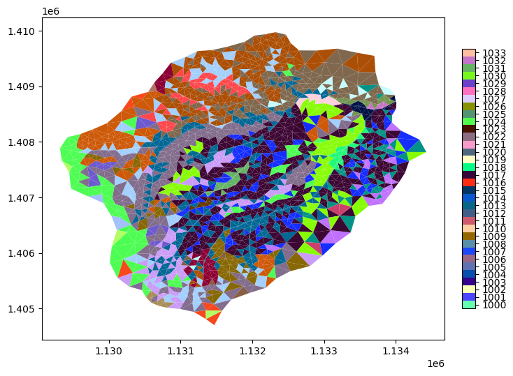
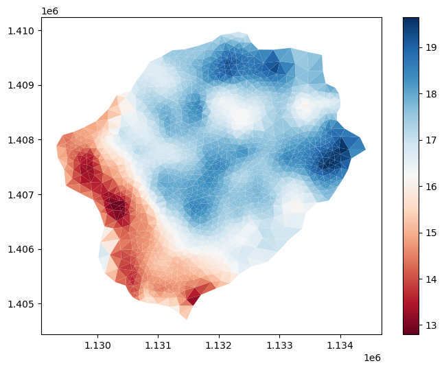
Depth to Bedrock from SoilGrids

dtb = sources['depth to bedrock'].getDataset(watershed.exterior, watershed.crs)['band_1']

# the SoilGrids dataset is in cm --> convert to meters
dtb.values = dtb.values/100.

2025-08-29 17:27:52,495 - root - INFO: Incoming shape area = 0.0016040429015210392
2025-08-29 17:27:52,496 - root - INFO: ... buffering incoming shape by = 0.0020833330000016304
2025-08-29 17:27:52,496 - root - INFO: ... buffered shape area = 0.00196035495453784

# map to the mesh
m2.cell_data['dtb'] = watershed_workflow.getDatasetOnMesh(m2, dtb, method='linear')

gons = m2.plot(facecolors=m2.cell_data['dtb'], cmap='RdBu', edgecolors=None)
plt.show()

GLHYMPs Geology

glhymps = sources['geologic structure'].getShapesByGeometry(watershed.exterior.buffer(1000), watershed.crs, out_crs=crs)
glhymps = watershed_workflow.soil_properties.mangleGLHYMPSProperties(glhymps,
                                              min_porosity=min_porosity, 
                                              max_permeability=max_permeability, 
                                              max_vg_alpha=max_vg_alpha)

# intersect with the buffered geometry -- don't keep extras
glhymps = glhymps[glhymps.intersects(watershed.exterior.buffer(10))]
glhymps

2025-08-29 17:27:52,723 - root - INFO: fixing column: geometry

	ID	name	source	permeability [m^2]	logk_stdev [-]	porosity [-]	van Genuchten alpha [Pa^-1]	van Genuchten n [-]	residual saturation [-]	geometry
1	1793338	GLHYMPS-1793338	GLHYMPS	3.019952e-11	1.61	0.05	0.001	2.0	0.01	MULTIPOLYGON (((1060059.466 1375224.917, 10600...

# quality check -- make sure glymps shapes cover the watershed
print(glhymps.union_all().contains(watershed.exterior))
glhymps

True

	ID	name	source	permeability [m^2]	logk_stdev [-]	porosity [-]	van Genuchten alpha [Pa^-1]	van Genuchten n [-]	residual saturation [-]	geometry
1	1793338	GLHYMPS-1793338	GLHYMPS	3.019952e-11	1.61	0.05	0.001	2.0	0.01	MULTIPOLYGON (((1060059.466 1375224.917, 10600...

# clean the data
glhymps.pop('logk_stdev [-]')

assert glhymps['porosity [-]'][:].min() >= min_porosity
assert glhymps['permeability [m^2]'][:].max() <= max_permeability
assert glhymps['van Genuchten alpha [Pa^-1]'][:].max() <= max_vg_alpha

glhymps.isna().any()

ID                             False
name                           False
source                         False
permeability [m^2]             False
porosity [-]                   False
van Genuchten alpha [Pa^-1]    False
van Genuchten n [-]            False
residual saturation [-]        False
geometry                       False
dtype: bool

# note that for larger areas there are often common regions -- two labels with the same properties -- no need to duplicate those with identical values.
def reindex_remove_duplicates(df, index):
    """Removes duplicates, creating a new index and saving the old index as tuples of duplicate values. In place!"""
    if index is not None:
        if index in df:
            df.set_index(index, drop=True, inplace=True)
    
    index_name = df.index.name

    # identify duplicate rows
    duplicates = list(df.groupby(list(df)).apply(lambda x: tuple(x.index)))

    # order is preserved
    df.drop_duplicates(inplace=True)
    df.reset_index(inplace=True)
    df[index_name] = duplicates
    return

reindex_remove_duplicates(glhymps, 'ID')
glhymps

	ID	name	source	permeability [m^2]	porosity [-]	van Genuchten alpha [Pa^-1]	van Genuchten n [-]	residual saturation [-]	geometry
0	(1793338,)	GLHYMPS-1793338	GLHYMPS	3.019952e-11	0.05	0.001	2.0	0.01	MULTIPOLYGON (((1060059.466 1375224.917, 10600...

# Compute the geo color of each cell of the mesh
geology_color_glhymps = watershed_workflow.getShapePropertiesOnMesh(m2, glhymps, 'index', 
                                                         resolution=50, nodata=-999)

# retain only the unique values of geology that actually appear in our cell mesh
unique_geology_colors = list(np.unique(geology_color_glhymps))
if -999 in unique_geology_colors:
    unique_geology_colors.remove(-999)

# retain only the unique values of geology_color
glhymps = glhymps.loc[unique_geology_colors]

# renumber the ones we know will appear with an ATS ID using ATS conventions
glhymps['ATS ID'] = range(100, 100+len(unique_geology_colors))
glhymps['TMP_ID'] = glhymps.index
glhymps.reset_index(drop=True, inplace=True)
glhymps.set_index('ATS ID', drop=True, inplace=True)

# create a new geology color using the ATS IDs
geology_color = -np.ones_like(geology_color_glhymps)
for ats_ID, tmp_ID in zip(glhymps.index, glhymps.TMP_ID):
    geology_color[np.where(geology_color_glhymps == tmp_ID)] = ats_ID

glhymps.pop('TMP_ID')

m2.cell_data['geology_color'] = geology_color
                            

geology_color_glhymps.min()

<xarray.DataArray 'index' ()> Size: 8B
array(0)

xarray.DataArray

'index'

• 0

  array(0)

• Coordinates: (0)
• Indexes: (0)
• Attributes: (0)

Combine to form a complete subsurface dataset

bedrock = watershed_workflow.soil_properties.getDefaultBedrockProperties()

# merge the properties databases
subsurface_props = pd.concat([glhymps, nrcs, bedrock])

# save the properties to disk for use in generating input file
output_filenames['subsurface_properties'] = toOutput(f'{name}_subsurface_properties.csv')
subsurface_props.to_csv(output_filenames['subsurface_properties'])
subsurface_props

	ID	name	source	permeability [m^2]	porosity [-]	van Genuchten alpha [Pa^-1]	van Genuchten n [-]	residual saturation [-]	geometry	mukey	thickness [m]
100	(1793338,)	GLHYMPS-1793338	GLHYMPS	3.019952e-11	0.050000	0.001000	2.000000	0.010000	MULTIPOLYGON (((1060059.466 1375224.917, 10600...	NaN	NaN
1000	545800	NRCS-545800	NRCS	3.429028e-15	0.307246	0.000139	1.470755	0.177165	MULTIPOLYGON (((1131335.296 1404750.906, 11313...	545800.0	2.03
1001	545803	NRCS-545803	NRCS	2.800000e-12	0.379163	0.000150	1.491087	0.172412	MULTIPOLYGON (((1130760.995 1408224.107, 11307...	545803.0	2.03
1002	545805	NRCS-545805	NRCS	2.800000e-12	0.384877	0.000083	1.468789	0.177122	MULTIPOLYGON (((1134255.698 1405132.204, 11342...	545805.0	2.03
1003	545806	NRCS-545806	NRCS	2.800000e-12	0.384877	0.000083	1.468789	0.177122	MULTIPOLYGON (((1134180.798 1405169.304, 11341...	545806.0	2.03
1004	545807	NRCS-545807	NRCS	2.800000e-12	0.384877	0.000083	1.468789	0.177122	MULTIPOLYGON (((1131255.496 1405664.406, 11312...	545807.0	2.03
1005	545811	NRCS-545811	NRCS	1.830706e-12	0.329821	0.000166	1.473045	0.185628	MULTIPOLYGON (((1130078.796 1404597.506, 11300...	545811.0	2.03
1006	545813	NRCS-545813	NRCS	6.219065e-14	0.349442	0.000127	1.445858	0.183468	MULTIPOLYGON (((1132919.997 1405040.305, 11329...	545813.0	2.03
1007	545814	NRCS-545814	NRCS	6.060887e-14	0.346424	0.000125	1.445793	0.183216	MULTIPOLYGON (((1131226.596 1404721.006, 11312...	545814.0	2.03
1008	545815	NRCS-545815	NRCS	3.794887e-14	0.319402	0.000162	1.498482	0.177808	MULTIPOLYGON (((1131297.396 1404750.606, 11313...	545815.0	2.03
1009	545818	NRCS-545818	NRCS	2.800000e-12	0.305511	0.000151	1.479294	0.176724	MULTIPOLYGON (((1129829.018 1404481.296, 11298...	545818.0	2.03
1010	545819	NRCS-545819	NRCS	2.800000e-12	0.313860	0.000149	1.469380	0.179179	MULTIPOLYGON (((1130832.496 1405209.106, 11308...	545819.0	2.03
1011	545820	NRCS-545820	NRCS	2.800000e-12	0.305511	0.000151	1.479294	0.176724	MULTIPOLYGON (((1130594.795 1406194.606, 11305...	545820.0	2.03
1012	545829	NRCS-545829	NRCS	2.091075e-12	0.421416	0.000131	1.409385	0.195475	MULTIPOLYGON (((1132541.183 1404841.203, 11325...	545829.0	2.03
1013	545830	NRCS-545830	NRCS	1.689101e-12	0.420388	0.000132	1.409349	0.195431	MULTIPOLYGON (((1132031.497 1405039.905, 11320...	545830.0	2.03
1014	545831	NRCS-545831	NRCS	1.729105e-12	0.418625	0.000134	1.409332	0.195360	MULTIPOLYGON (((1130650.695 1406946.307, 11306...	545831.0	2.03
1015	545835	NRCS-545835	NRCS	9.069462e-13	0.375338	0.000125	1.404309	0.202983	MULTIPOLYGON (((1131130.296 1406792.506, 11311...	545835.0	2.03
1016	545836	NRCS-545836	NRCS	8.686821e-13	0.410934	0.000118	1.356194	0.225964	MULTIPOLYGON (((1133372.798 1405277.705, 11333...	545836.0	2.03
1017	545837	NRCS-545837	NRCS	9.140653e-13	0.353400	0.000117	1.368452	0.219777	MULTIPOLYGON (((1132492.397 1405272.505, 11325...	545837.0	2.03
1018	545838	NRCS-545838	NRCS	9.090539e-13	0.348524	0.000114	1.359591	0.224883	MULTIPOLYGON (((1132692.297 1406223.605, 11326...	545838.0	2.03
1019	545842	NRCS-545842	NRCS	9.952892e-13	0.386946	0.000142	1.434838	0.193278	MULTIPOLYGON (((1132238.796 1408684.207, 11322...	545842.0	2.03
1020	545843	NRCS-545843	NRCS	9.952892e-13	0.387980	0.000118	1.409272	0.200565	MULTIPOLYGON (((1130711.995 1408154.207, 11307...	545843.0	2.03
1021	545853	NRCS-545853	NRCS	1.811809e-12	0.466299	0.000127	1.464370	0.174940	MULTIPOLYGON (((1130816.796 1405093.006, 11308...	545853.0	2.03
1022	545854	NRCS-545854	NRCS	1.811809e-12	0.466299	0.000127	1.464370	0.174940	MULTIPOLYGON (((1130252.496 1404576.306, 11302...	545854.0	2.03
1023	545855	NRCS-545855	NRCS	6.238368e-12	0.235555	0.000247	1.928427	0.149582	POLYGON ((1133569.697 1408334.306, 1133563.297...	545855.0	2.03
1024	545857	NRCS-545857	NRCS	4.981053e-15	0.405556	0.000147	1.484106	0.175471	MULTIPOLYGON (((1132073.397 1404858.905, 11320...	545857.0	2.03
1025	545859	NRCS-545859	NRCS	1.107558e-12	0.265930	0.000108	1.389431	0.209607	MULTIPOLYGON (((1133532.297 1408393.806, 11335...	545859.0	2.03
1026	545860	NRCS-545860	NRCS	1.035014e-12	0.269704	0.000105	1.390548	0.210433	MULTIPOLYGON (((1133109.197 1406512.605, 11331...	545860.0	2.03
1027	545861	NRCS-545861	NRCS	1.968721e-12	0.309901	0.000117	1.404424	0.202264	MULTIPOLYGON (((1133264.497 1408640.506, 11332...	545861.0	2.03
1028	545874	NRCS-545874	NRCS	1.023505e-12	0.365616	0.000135	1.395264	0.208675	MULTIPOLYGON (((1133454.498 1405357.905, 11334...	545874.0	2.03
1029	545875	NRCS-545875	NRCS	1.023505e-12	0.365616	0.000135	1.395264	0.208675	MULTIPOLYGON (((1132812.997 1406047.305, 11328...	545875.0	2.03
1030	545876	NRCS-545876	NRCS	2.800000e-12	0.324877	0.000141	1.449088	0.184037	MULTIPOLYGON (((1134517.198 1407050.505, 11345...	545876.0	2.03
1031	545878	NRCS-545878	NRCS	2.282599e-12	0.364041	0.000125	1.416495	0.196924	MULTIPOLYGON (((1129854.195 1404493.006, 11299...	545878.0	1.85
1032	545882	NRCS-545882	NRCS	2.800000e-12	0.280000	0.000091	1.439689	0.184498	POLYGON ((1133621.697 1408540.806, 1133603.497...	545882.0	2.03
1033	545885	NRCS-545885	NRCS	2.800000e-12	0.326502	0.000183	1.574297	0.165660	MULTIPOLYGON (((1130139.195 1406476.107, 11301...	545885.0	2.03
999	999	bedrock	n/a	1.000000e-16	0.050000	0.000019	3.000000	0.010000	None	NaN	NaN

Extrude the 2D Mesh to make a 3D mesh

# set the floor of the domain as max DTB
dtb_max = np.nanmax(m2.cell_data['dtb'].values)
m2.cell_data['dtb'] = m2.cell_data['dtb'].fillna(dtb_max)

print(f'total thickness: {dtb_max} m')
total_thickness = 50.

total thickness: 19.647739130592548 m

# Generate a dz structure for the top 2m of soil
#
# here we try for 10 cells, starting at 5cm at the top and going to 50cm at the bottom of the 2m thick soil
dzs, res = watershed_workflow.mesh.optimizeDzs(0.05, 0.5, 2, 10)
print(dzs)
print(sum(dzs))

[0.05447108 0.07161305 0.11027281 0.17443206 0.26441087 0.36782677
 0.45697337 0.49999999]
2.0000000000000004

# this looks like it would work out, with rounder numbers:
dzs_soil = [0.05, 0.05, 0.05, 0.12, 0.23, 0.5, 0.5, 0.5]
print(sum(dzs_soil))

2.0

# 50m total thickness, minus 2m soil thickness, leaves us with 48 meters to make up.
# optimize again...
dzs2, res2 = watershed_workflow.mesh.optimizeDzs(1, 10, 48, 8)
print(dzs2)
print(sum(dzs2))

# how about...
dzs_geo = [1.0, 2.0, 4.0, 8.0, 11, 11, 11]
print(dzs_geo)
print(sum(dzs_geo))

[2.71113048 5.85796948 9.43304714 9.99786869 9.99998875 9.99999546]
48.0
[1.0, 2.0, 4.0, 8.0, 11, 11, 11]
48.0

# layer extrusion
DTB = m2.cell_data['dtb'].values
soil_color = m2.cell_data['soil_color'].values
geo_color = m2.cell_data['geology_color'].values
soil_thickness = m2.cell_data['soil thickness'].values


# -- data structures needed for extrusion
layer_types = []
layer_data = []
layer_ncells = []
layer_mat_ids = []

# -- soil layer --
depth = 0
for dz in dzs_soil:
    depth += 0.5 * dz
    layer_types.append('constant')
    layer_data.append(dz)
    layer_ncells.append(1)
    
    # use glhymps params
    br_or_geo = np.where(depth < DTB, geo_color, 999)
    soil_or_br_or_geo = np.where(np.bitwise_and(soil_color > 0, depth < soil_thickness),
                                 soil_color,
                                 br_or_geo)

    layer_mat_ids.append(soil_or_br_or_geo)
    depth += 0.5 * dz
    
# -- geologic layer --
for dz in dzs_geo:
    depth += 0.5 * dz
    layer_types.append('constant')
    layer_data.append(dz)
    layer_ncells.append(1)
    
    geo_or_br = np.where(depth < DTB, geo_color, 999)

    layer_mat_ids.append(geo_or_br)
    depth += 0.5 * dz

# print the summary
watershed_workflow.mesh.Mesh3D.summarizeExtrusion(layer_types, layer_data, 
                                            layer_ncells, layer_mat_ids)

# downselect subsurface properties to only those that are used
layer_mat_id_used = list(np.unique(np.array(layer_mat_ids)))
subsurface_props_used = subsurface_props.loc[layer_mat_id_used]
subsurface_props_used

2025-08-29 17:27:53,356 - root - INFO: Cell summary:
2025-08-29 17:27:53,357 - root - INFO: ------------------------------------------------------------
2025-08-29 17:27:53,357 - root - INFO: l_id	| c_id	|mat_id	| dz		| z_top
2025-08-29 17:27:53,357 - root - INFO: ------------------------------------------------------------
2025-08-29 17:27:53,357 - root - INFO:  00 	| 00 	| 1008 	|   0.050000 	|   0.000000
2025-08-29 17:27:53,358 - root - INFO:  01 	| 01 	| 1008 	|   0.050000 	|   0.050000
2025-08-29 17:27:53,358 - root - INFO:  02 	| 02 	| 1008 	|   0.050000 	|   0.100000
2025-08-29 17:27:53,358 - root - INFO:  03 	| 03 	| 1008 	|   0.120000 	|   0.150000
2025-08-29 17:27:53,359 - root - INFO:  04 	| 04 	| 1008 	|   0.230000 	|   0.270000
2025-08-29 17:27:53,359 - root - INFO:  05 	| 05 	| 1008 	|   0.500000 	|   0.500000
2025-08-29 17:27:53,359 - root - INFO:  06 	| 06 	| 1008 	|   0.500000 	|   1.000000
2025-08-29 17:27:53,359 - root - INFO:  07 	| 07 	| 1008 	|   0.500000 	|   1.500000
2025-08-29 17:27:53,360 - root - INFO:  08 	| 08 	|  100 	|   1.000000 	|   2.000000
2025-08-29 17:27:53,360 - root - INFO:  09 	| 09 	|  100 	|   2.000000 	|   3.000000
2025-08-29 17:27:53,360 - root - INFO:  10 	| 10 	|  100 	|   4.000000 	|   5.000000
2025-08-29 17:27:53,360 - root - INFO:  11 	| 11 	|  100 	|   8.000000 	|   9.000000
2025-08-29 17:27:53,360 - root - INFO:  12 	| 12 	|  999 	|  11.000000 	|  17.000000
2025-08-29 17:27:53,360 - root - INFO:  13 	| 13 	|  999 	|  11.000000 	|  28.000000
2025-08-29 17:27:53,361 - root - INFO:  14 	| 14 	|  999 	|  11.000000 	|  39.000000

	ID	name	source	permeability [m^2]	porosity [-]	van Genuchten alpha [Pa^-1]	van Genuchten n [-]	residual saturation [-]	geometry	mukey	thickness [m]
100	(1793338,)	GLHYMPS-1793338	GLHYMPS	3.019952e-11	0.050000	0.001000	2.000000	0.010000	MULTIPOLYGON (((1060059.466 1375224.917, 10600...	NaN	NaN
999	999	bedrock	n/a	1.000000e-16	0.050000	0.000019	3.000000	0.010000	None	NaN	NaN
1000	545800	NRCS-545800	NRCS	3.429028e-15	0.307246	0.000139	1.470755	0.177165	MULTIPOLYGON (((1131335.296 1404750.906, 11313...	545800.0	2.03
1001	545803	NRCS-545803	NRCS	2.800000e-12	0.379163	0.000150	1.491087	0.172412	MULTIPOLYGON (((1130760.995 1408224.107, 11307...	545803.0	2.03
1002	545805	NRCS-545805	NRCS	2.800000e-12	0.384877	0.000083	1.468789	0.177122	MULTIPOLYGON (((1134255.698 1405132.204, 11342...	545805.0	2.03
1003	545806	NRCS-545806	NRCS	2.800000e-12	0.384877	0.000083	1.468789	0.177122	MULTIPOLYGON (((1134180.798 1405169.304, 11341...	545806.0	2.03
1004	545807	NRCS-545807	NRCS	2.800000e-12	0.384877	0.000083	1.468789	0.177122	MULTIPOLYGON (((1131255.496 1405664.406, 11312...	545807.0	2.03
1005	545811	NRCS-545811	NRCS	1.830706e-12	0.329821	0.000166	1.473045	0.185628	MULTIPOLYGON (((1130078.796 1404597.506, 11300...	545811.0	2.03
1006	545813	NRCS-545813	NRCS	6.219065e-14	0.349442	0.000127	1.445858	0.183468	MULTIPOLYGON (((1132919.997 1405040.305, 11329...	545813.0	2.03
1007	545814	NRCS-545814	NRCS	6.060887e-14	0.346424	0.000125	1.445793	0.183216	MULTIPOLYGON (((1131226.596 1404721.006, 11312...	545814.0	2.03
1008	545815	NRCS-545815	NRCS	3.794887e-14	0.319402	0.000162	1.498482	0.177808	MULTIPOLYGON (((1131297.396 1404750.606, 11313...	545815.0	2.03
1009	545818	NRCS-545818	NRCS	2.800000e-12	0.305511	0.000151	1.479294	0.176724	MULTIPOLYGON (((1129829.018 1404481.296, 11298...	545818.0	2.03
1010	545819	NRCS-545819	NRCS	2.800000e-12	0.313860	0.000149	1.469380	0.179179	MULTIPOLYGON (((1130832.496 1405209.106, 11308...	545819.0	2.03
1011	545820	NRCS-545820	NRCS	2.800000e-12	0.305511	0.000151	1.479294	0.176724	MULTIPOLYGON (((1130594.795 1406194.606, 11305...	545820.0	2.03
1012	545829	NRCS-545829	NRCS	2.091075e-12	0.421416	0.000131	1.409385	0.195475	MULTIPOLYGON (((1132541.183 1404841.203, 11325...	545829.0	2.03
1013	545830	NRCS-545830	NRCS	1.689101e-12	0.420388	0.000132	1.409349	0.195431	MULTIPOLYGON (((1132031.497 1405039.905, 11320...	545830.0	2.03
1014	545831	NRCS-545831	NRCS	1.729105e-12	0.418625	0.000134	1.409332	0.195360	MULTIPOLYGON (((1130650.695 1406946.307, 11306...	545831.0	2.03
1015	545835	NRCS-545835	NRCS	9.069462e-13	0.375338	0.000125	1.404309	0.202983	MULTIPOLYGON (((1131130.296 1406792.506, 11311...	545835.0	2.03
1016	545836	NRCS-545836	NRCS	8.686821e-13	0.410934	0.000118	1.356194	0.225964	MULTIPOLYGON (((1133372.798 1405277.705, 11333...	545836.0	2.03
1017	545837	NRCS-545837	NRCS	9.140653e-13	0.353400	0.000117	1.368452	0.219777	MULTIPOLYGON (((1132492.397 1405272.505, 11325...	545837.0	2.03
1018	545838	NRCS-545838	NRCS	9.090539e-13	0.348524	0.000114	1.359591	0.224883	MULTIPOLYGON (((1132692.297 1406223.605, 11326...	545838.0	2.03
1019	545842	NRCS-545842	NRCS	9.952892e-13	0.386946	0.000142	1.434838	0.193278	MULTIPOLYGON (((1132238.796 1408684.207, 11322...	545842.0	2.03
1020	545843	NRCS-545843	NRCS	9.952892e-13	0.387980	0.000118	1.409272	0.200565	MULTIPOLYGON (((1130711.995 1408154.207, 11307...	545843.0	2.03
1021	545853	NRCS-545853	NRCS	1.811809e-12	0.466299	0.000127	1.464370	0.174940	MULTIPOLYGON (((1130816.796 1405093.006, 11308...	545853.0	2.03
1022	545854	NRCS-545854	NRCS	1.811809e-12	0.466299	0.000127	1.464370	0.174940	MULTIPOLYGON (((1130252.496 1404576.306, 11302...	545854.0	2.03
1023	545855	NRCS-545855	NRCS	6.238368e-12	0.235555	0.000247	1.928427	0.149582	POLYGON ((1133569.697 1408334.306, 1133563.297...	545855.0	2.03
1024	545857	NRCS-545857	NRCS	4.981053e-15	0.405556	0.000147	1.484106	0.175471	MULTIPOLYGON (((1132073.397 1404858.905, 11320...	545857.0	2.03
1025	545859	NRCS-545859	NRCS	1.107558e-12	0.265930	0.000108	1.389431	0.209607	MULTIPOLYGON (((1133532.297 1408393.806, 11335...	545859.0	2.03
1026	545860	NRCS-545860	NRCS	1.035014e-12	0.269704	0.000105	1.390548	0.210433	MULTIPOLYGON (((1133109.197 1406512.605, 11331...	545860.0	2.03
1027	545861	NRCS-545861	NRCS	1.968721e-12	0.309901	0.000117	1.404424	0.202264	MULTIPOLYGON (((1133264.497 1408640.506, 11332...	545861.0	2.03
1028	545874	NRCS-545874	NRCS	1.023505e-12	0.365616	0.000135	1.395264	0.208675	MULTIPOLYGON (((1133454.498 1405357.905, 11334...	545874.0	2.03
1029	545875	NRCS-545875	NRCS	1.023505e-12	0.365616	0.000135	1.395264	0.208675	MULTIPOLYGON (((1132812.997 1406047.305, 11328...	545875.0	2.03
1030	545876	NRCS-545876	NRCS	2.800000e-12	0.324877	0.000141	1.449088	0.184037	MULTIPOLYGON (((1134517.198 1407050.505, 11345...	545876.0	2.03
1031	545878	NRCS-545878	NRCS	2.282599e-12	0.364041	0.000125	1.416495	0.196924	MULTIPOLYGON (((1129854.195 1404493.006, 11299...	545878.0	1.85
1032	545882	NRCS-545882	NRCS	2.800000e-12	0.280000	0.000091	1.439689	0.184498	POLYGON ((1133621.697 1408540.806, 1133603.497...	545882.0	2.03
1033	545885	NRCS-545885	NRCS	2.800000e-12	0.326502	0.000183	1.574297	0.165660	MULTIPOLYGON (((1130139.195 1406476.107, 11301...	545885.0	2.03

# extrude
m3 = watershed_workflow.mesh.Mesh3D.extruded_Mesh2D(m2, layer_types, layer_data, 
                                             layer_ncells, layer_mat_ids)

print('2D labeled sets')
print('---------------')
for ls in m2.labeled_sets:
    print(f'{ls.setid} : {ls.entity} : {len(ls.ent_ids)} : "{ls.name}"')

print('')
print('Extruded 3D labeled sets')
print('------------------------')
for ls in m3.labeled_sets:
    print(f'{ls.setid} : {ls.entity} : {len(ls.ent_ids)} : "{ls.name}"')

print('')
print('Extruded 3D side sets')
print('---------------------')
for ls in m3.side_sets:
    print(f'{ls.setid} : FACE : {len(ls.cell_list)} : "{ls.name}"')
    

2D labeled sets
---------------
10000 : CELL : 2683 : "0"
10001 : CELL : 2683 : "0 surface"
10002 : FACE : 76 : "0 boundary"
10003 : FACE : 5 : "0 outlet"
10004 : FACE : 5 : "surface domain outlet"
10005 : CELL : 190 : "river corridor 0 surface"
10006 : CELL : 16 : "stream order 3"
10007 : CELL : 48 : "stream order 2"
10008 : CELL : 126 : "stream order 1"
21 : CELL : 104 : "Developed, Open Space"
22 : CELL : 5 : "Developed, Low Intensity"
23 : CELL : 1 : "Developed, Medium Intensity"
41 : CELL : 1393 : "Deciduous Forest"
42 : CELL : 43 : "Evergreen Forest"
43 : CELL : 1133 : "Mixed Forest"
81 : CELL : 4 : "Pasture/Hay"

Extruded 3D labeled sets
------------------------
10000 : CELL : 40245 : "0"

Extruded 3D side sets
---------------------
1 : FACE : 2683 : "bottom"
2 : FACE : 2683 : "surface"
3 : FACE : 1140 : "external sides"
10001 : FACE : 2683 : "0 surface"
10002 : FACE : 1140 : "0 boundary"
10003 : FACE : 75 : "0 outlet"
10004 : FACE : 75 : "surface domain outlet"
10005 : FACE : 190 : "river corridor 0 surface"
10006 : FACE : 16 : "stream order 3"
10007 : FACE : 48 : "stream order 2"
10008 : FACE : 126 : "stream order 1"
21 : FACE : 104 : "Developed, Open Space"
22 : FACE : 5 : "Developed, Low Intensity"
23 : FACE : 1 : "Developed, Medium Intensity"
41 : FACE : 1393 : "Deciduous Forest"
42 : FACE : 43 : "Evergreen Forest"
43 : FACE : 1133 : "Mixed Forest"
81 : FACE : 4 : "Pasture/Hay"

# save the mesh to disk
output_filenames['mesh'] = toOutput(f'{name}.exo')
try:
    os.remove(output_filenames['mesh'])
except FileNotFoundError:
    pass
m3.writeExodus(output_filenames['mesh'])

You are using exodus.py v 1.20.10 (seacas-py3), a python wrapper of some of the exodus library.

Copyright (c) 2013, 2014, 2015, 2016, 2017, 2018, 2019, 2020, 2021 National Technology &
Engineering Solutions of Sandia, LLC (NTESS).  Under the terms of
Contract DE-NA0003525 with NTESS, the U.S. Government retains certain
rights in this software.

Opening exodus file: /home/ecoon/code/watershed_workflow/repos/master/examples/Coweeta/output_data/Coweeta.exo

2025-08-29 17:27:53,697 - root - INFO: adding side set: 1
2025-08-29 17:27:53,703 - root - INFO: adding side set: 2
2025-08-29 17:27:53,706 - root - INFO: adding side set: 3
2025-08-29 17:27:53,708 - root - INFO: adding side set: 10001
2025-08-29 17:27:53,710 - root - INFO: adding side set: 10002
2025-08-29 17:27:53,712 - root - INFO: adding side set: 10003
2025-08-29 17:27:53,713 - root - INFO: adding side set: 10004
2025-08-29 17:27:53,714 - root - INFO: adding side set: 10005
2025-08-29 17:27:53,715 - root - INFO: adding side set: 10006
2025-08-29 17:27:53,716 - root - INFO: adding side set: 10007
2025-08-29 17:27:53,718 - root - INFO: adding side set: 10008
2025-08-29 17:27:53,719 - root - INFO: adding side set: 21
2025-08-29 17:27:53,720 - root - INFO: adding side set: 22
2025-08-29 17:27:53,721 - root - INFO: adding side set: 23
2025-08-29 17:27:53,722 - root - INFO: adding side set: 41
2025-08-29 17:27:53,724 - root - INFO: adding side set: 42
2025-08-29 17:27:53,725 - root - INFO: adding side set: 43
2025-08-29 17:27:53,727 - root - INFO: adding side set: 81
2025-08-29 17:27:53,728 - root - WARNING: not writing elem_set: 10000 because this exodus installation does not write element sets

Closing exodus file: /home/ecoon/code/watershed_workflow/repos/master/examples/Coweeta/output_data/Coweeta.exo

Meteorological forcing dataset

# download the data -- note it is hourly!
met_data_raw = sources['meteorology'].getDataset(watershed.exterior, crs, start_leap, end_leap)

# convert it to daily mean immediately
met_data_raw_daily = met_data_raw.resample(time=datetime.timedelta(hours=24)).mean()

# also, note that we sampled from 8/1 to 8/1, meaning we have an extra day now.
met_data_raw_daily = met_data_raw_daily.isel({'time' : slice(0, -1)})
print(f'Total days: {len(met_data_raw_daily['time'])}')

2025-08-29 17:27:53,758 - root - INFO: Incoming shape area = 0.0016040429015210392
2025-08-29 17:27:53,758 - root - INFO: ... buffering incoming shape by = 0.00833333
2025-08-29 17:27:53,759 - root - INFO: ... buffered shape area = 0.0031753726729616284

Variable size: 99.0 TB
<xarray.Dataset> Size: 99TB
Dimensions:              (time: 43824, latitude: 4201, longitude: 8401)
Coordinates:
  * latitude             (latitude) float64 34kB 20.0 20.01 20.02 ... 54.99 55.0
  * longitude            (longitude) float64 67kB -130.0 -130.0 ... -60.01 -60.0
  * time                 (time) datetime64[ns] 351kB 2010-01-01 ... 2014-12-3...
Data variables:
    APCP_surface         (time, latitude, longitude) float64 12TB dask.array<chunksize=(144, 128, 256), meta=np.ndarray>
    DLWRF_surface        (time, latitude, longitude) float64 12TB dask.array<chunksize=(144, 128, 256), meta=np.ndarray>
    DSWRF_surface        (time, latitude, longitude) float64 12TB dask.array<chunksize=(144, 128, 256), meta=np.ndarray>
    PRES_surface         (time, latitude, longitude) float64 12TB dask.array<chunksize=(144, 128, 256), meta=np.ndarray>
    SPFH_2maboveground   (time, latitude, longitude) float64 12TB dask.array<chunksize=(144, 128, 256), meta=np.ndarray>
    TMP_2maboveground    (time, latitude, longitude) float64 12TB dask.array<chunksize=(144, 128, 256), meta=np.ndarray>
    UGRD_10maboveground  (time, latitude, longitude) float64 12TB dask.array<chunksize=(144, 128, 256), meta=np.ndarray>
    VGRD_10maboveground  (time, latitude, longitude) float64 12TB dask.array<chunksize=(144, 128, 256), meta=np.ndarray>
Subsetting:
  lon: (np.float64(-83.4863), np.float64(-83.4138))
  lat: (np.float64(35.0197), np.float64(35.0821))
Variable size: 0.177 GB
Total days: 1461

# AORC is a non-projected dataset in lat-lon
# warp it to projected
met_data_warped = watershed_workflow.warp.dataset(met_data_raw_daily, crs, 'bilinear')

# convert and write ATS format for transient run
met_data_transient = watershed_workflow.meteorology.convertAORCToATS(met_data_warped)
met_data_transient

2025-08-29 17:34:54,371 - root - INFO: Converting AORC to ATS met input

<xarray.Dataset> Size: 8MB
Dimensions:                                (x: 9, y: 9, time: 1461)
Coordinates:
  * x                                      (x) float64 72B 1.128e+06 ... 1.13...
  * y                                      (y) float64 72B 1.41e+06 ... 1.404...
  * time                                   (time) object 12kB 2010-08-01 00:0...
    spatial_ref                            int64 8B 0
Data variables:
    air temperature [K]                    (time, y, x) float64 947kB nan ......
    incoming shortwave radiation [W m^-2]  (time, y, x) float64 947kB nan ......
    incoming longwave radiation [W m^-2]   (time, y, x) float64 947kB nan ......
    vapor pressure air [Pa]                (time, y, x) float64 947kB nan ......
    wind speed [m s^-1]                    (time, y, x) float64 947kB nan ......
    precipitation total [m s^-1]           (time, y, x) float64 947kB nan ......
    precipitation rain [m s^-1]            (time, y, x) float64 947kB 0.0 ......
    precipitation snow [m SWE s^-1]        (time, y, x) float64 947kB 0.0 ......
Attributes:
    name:                             AORC v1.1
    source:                           NOAA AWS S3 Zarr
    wind speed reference height [m]:  10.0

xarray.Dataset

• Dimensions:
  • x: 9
  • y: 9
  • time: 1461
• Coordinates: (4)
  • x
    (x)
    float64
    1.128e+06 1.129e+06 ... 1.135e+06

    array([1128418.497769, 1129244.157954, 1130069.818139, 1130895.478324,
           1131721.138509, 1132546.798694, 1133372.458879, 1134198.119063,
           1135023.779248])

  • y
    (y)
    float64
    1.41e+06 1.41e+06 ... 1.404e+06

    array([1410426.807656, 1409601.147471, 1408775.487286, 1407949.827101,
           1407124.166916, 1406298.506731, 1405472.846546, 1404647.186362,
           1403821.526177])

  • time
    (time)
    object
    2010-08-01 00:00:00 ... 2014-07-...

    array([cftime.DatetimeGregorian(2010, 8, 1, 0, 0, 0, 0, has_year_zero=False),
           cftime.DatetimeGregorian(2010, 8, 2, 0, 0, 0, 0, has_year_zero=False),
           cftime.DatetimeGregorian(2010, 8, 3, 0, 0, 0, 0, has_year_zero=False),
           ...,
           cftime.DatetimeGregorian(2014, 7, 29, 0, 0, 0, 0, has_year_zero=False),
           cftime.DatetimeGregorian(2014, 7, 30, 0, 0, 0, 0, has_year_zero=False),
           cftime.DatetimeGregorian(2014, 7, 31, 0, 0, 0, 0, has_year_zero=False)],
          shape=(1461,), dtype=object)

  • spatial_ref
    ()
    int64
    0

    crs_wkt :

    PROJCS["NAD83 / Conus Albers",GEOGCS["NAD83",DATUM["North_American_Datum_1983",SPHEROID["GRS 1980",6378137,298.257222101]],PRIMEM["Greenwich",0],UNIT["degree",0.0174532925199433,AUTHORITY["EPSG","9122"]],AUTHORITY["EPSG","4269"]],PROJECTION["Albers_Conic_Equal_Area"],PARAMETER["latitude_of_center",23],PARAMETER["longitude_of_center",-96],PARAMETER["standard_parallel_1",29.5],PARAMETER["standard_parallel_2",45.5],PARAMETER["false_easting",0],PARAMETER["false_northing",0],UNIT["metre",1],AXIS["Easting",EAST],AXIS["Northing",NORTH],AUTHORITY["EPSG","5070"]]

    semi_major_axis :

    6378137.0

    semi_minor_axis :

    6356752.314140356

    inverse_flattening :

    298.257222101

    reference_ellipsoid_name :

    GRS 1980

    longitude_of_prime_meridian :

    0.0

    prime_meridian_name :

    Greenwich

    geographic_crs_name :

    NAD83

    horizontal_datum_name :

    North American Datum 1983

    projected_crs_name :

    NAD83 / Conus Albers

    grid_mapping_name :

    albers_conical_equal_area

    standard_parallel :

    (29.5, 45.5)

    latitude_of_projection_origin :

    23.0

    longitude_of_central_meridian :

    -96.0

    false_easting :

    0.0

    false_northing :

    0.0

    spatial_ref :

    PROJCS["NAD83 / Conus Albers",GEOGCS["NAD83",DATUM["North_American_Datum_1983",SPHEROID["GRS 1980",6378137,298.257222101]],PRIMEM["Greenwich",0],UNIT["degree",0.0174532925199433,AUTHORITY["EPSG","9122"]],AUTHORITY["EPSG","4269"]],PROJECTION["Albers_Conic_Equal_Area"],PARAMETER["latitude_of_center",23],PARAMETER["longitude_of_center",-96],PARAMETER["standard_parallel_1",29.5],PARAMETER["standard_parallel_2",45.5],PARAMETER["false_easting",0],PARAMETER["false_northing",0],UNIT["metre",1],AXIS["Easting",EAST],AXIS["Northing",NORTH],AUTHORITY["EPSG","5070"]]

    GeoTransform :

    1128005.667676891 825.660184871774 0.0 1410839.6377481048 0.0 -825.660184871774

    array(0)

• Data variables: (8)
  • air temperature [K]
    (time, y, x)
    float64
    nan nan nan nan ... nan nan nan nan

    AORC_Contact :

    aorc.info@noaa.gov

    aorc_version :

    v1.1

    level :

    2 m above ground

    long_name :

    Temperature

    short_name :

    TMP_2maboveground

    units :

    K

    _FillValue :

    nan

    array([[[         nan,          nan,          nan, ..., 297.01970602,
             297.0831444 ,          nan],
            [295.94167108, 296.50383577, 296.12757939, ..., 296.75440842,
             297.13096262,          nan],
            [295.3993245 , 295.17070276, 295.83463549, ..., 296.62607068,
             296.95954862,          nan],
            ...,
            [         nan, 293.91887459, 294.6997662 , ..., 296.17648866,
             296.60396676, 296.42512912],
            [         nan, 294.05006792, 294.2927717 , ..., 295.89321231,
             296.46002704, 296.43080388],
            [         nan, 294.17285241, 294.52497602, ...,          nan,
                      nan,          nan]],
    
           [[         nan,          nan,          nan, ..., 297.92507297,
             297.97930708,          nan],
            [296.81250442, 297.37509095, 297.01270883, ..., 297.63772619,
             298.00608661,          nan],
            [296.25676657, 296.02620153, 296.69660671, ..., 297.48434224,
             297.80712355,          nan],
    ...
            [         nan, 287.0376977 , 287.8770312 , ..., 289.34518982,
             289.78373057, 289.53893142],
            [         nan, 287.15714635, 287.4767115 , ..., 289.10286409,
             289.64857275, 289.58986738],
            [         nan, 287.30639983, 287.71147867, ...,          nan,
                      nan,          nan]],
    
           [[         nan,          nan,          nan, ..., 290.98997339,
             291.05014031,          nan],
            [289.73750432, 290.24775584, 290.01553283, ..., 290.72499923,
             291.11652513,          nan],
            [289.27550538, 289.0710378 , 289.77788131, ..., 290.63232527,
             290.99474335,          nan],
            ...,
            [         nan, 287.85807709, 288.72918943, ..., 290.29459454,
             290.75829004, 290.50991846],
            [         nan, 287.97882898, 288.3217372 , ..., 290.03885199,
             290.59258422, 290.5449361 ],
            [         nan, 288.11993063, 288.54800749, ...,          nan,
                      nan,          nan]]], shape=(1461, 9, 9))

  • incoming shortwave radiation [W m^-2]
    (time, y, x)
    float64
    nan nan nan nan ... nan nan nan nan

    AORC_Contact :

    aorc.info@noaa.gov

    aorc_version :

    v1.1

    level :

    surface

    long_name :

    Downward Short-Wave Rad. Flux

    short_name :

    DSWRF_surface

    units :

    W/m^2

    _FillValue :

    nan

    array([[[         nan,          nan,          nan, ..., 203.52746326,
             203.86074155,          nan],
            [204.06250304, 203.86826562, 203.68504513, ..., 203.31827451,
             203.61590489,          nan],
            [203.90850339, 203.71363413, 203.54872553, ..., 203.3414665 ,
             203.70412531,          nan],
            ...,
            [         nan, 206.03030674, 205.91967235, ..., 205.56998821,
             205.75537814, 206.01362247],
            [         nan, 206.72910622, 206.61150919, ..., 206.21121133,
             206.34217607, 206.49227094],
            [         nan, 207.30743617, 207.07533473, ...,          nan,
                      nan,          nan]],
    
           [[         nan,          nan,          nan, ..., 294.57232092,
             294.54649641,          nan],
            [294.79583773, 294.79915689, 294.80084348, ..., 295.00279934,
             295.0825577 ,          nan],
            [295.17079339, 295.21364268, 295.24853735, ..., 295.42256857,
             295.46954324,          nan],
    ...
            [         nan, 305.72575035, 305.88691164, ..., 306.59186525,
             306.74627204, 306.94998082],
            [         nan, 306.39225118, 306.56833944, ..., 307.33693987,
             307.53384425, 307.65713503],
            [         nan, 306.90176494, 307.00762253, ...,          nan,
                      nan,          nan]],
    
           [[         nan,          nan,          nan, ..., 168.5108049 ,
             168.57401449,          nan],
            [168.40000251, 168.39612332, 168.35002198, ..., 168.32019285,
             168.3754381 ,          nan],
            [168.04178594, 168.05101374, 168.02684926, ..., 168.31296011,
             168.44778063,          nan],
            ...,
            [         nan, 169.09907391, 169.25455434, ..., 169.88349718,
             170.08588322, 170.2748666 ],
            [         nan, 169.44417723, 169.61043638, ..., 170.33390695,
             170.50220417, 170.63973606],
            [         nan, 169.71061163, 169.82735471, ...,          nan,
                      nan,          nan]]], shape=(1461, 9, 9))

  • incoming longwave radiation [W m^-2]
    (time, y, x)
    float64
    nan nan nan nan ... nan nan nan nan

    AORC_Contact :

    aorc.info@noaa.gov

    aorc_version :

    v1.1

    level :

    surface

    long_name :

    Downward Long-Wave Rad. Flux

    short_name :

    DLWRF_surface

    units :

    W/m^2

    _FillValue :

    nan

    array([[[         nan,          nan,          nan, ..., 403.91186279,
             404.13659658,          nan],
            [396.95833925, 400.2139669 , 398.38920439, ..., 402.37578494,
             404.29503098,          nan],
            [393.96204179, 392.86595127, 396.61381013, ..., 401.56040359,
             403.24434445,          nan],
            ...,
            [         nan, 386.04885264, 390.37865388, ..., 398.90571749,
             401.17959133, 400.13795876],
            [         nan, 386.7008737 , 388.17442333, ..., 397.36704634,
             400.42441987, 400.16620292],
            [         nan, 387.30934631, 389.3662748 , ...,          nan,
                      nan,          nan]],
    
           [[         nan,          nan,          nan, ..., 387.16758094,
             387.43593765,          nan],
            [380.25000567, 383.43379579, 381.70913509, ..., 385.46218959,
             387.3078604 ,          nan],
            [377.19679529, 376.19236498, 379.77552811, ..., 384.50237458,
             386.16883827,          nan],
    ...
            [         nan, 300.89288125, 304.59123151, ..., 311.39500914,
             313.29080793, 312.17583198],
            [         nan, 301.4370305 , 302.93928062, ..., 310.39428359,
             312.7046702 , 312.42895879],
            [         nan, 302.07541265, 303.94528856, ...,          nan,
                      nan,          nan]],
    
           [[         nan,          nan,          nan, ..., 353.59011138,
             353.77395986,          nan],
            [346.81667183, 349.45212651, 348.51813444, ..., 352.34645085,
             354.11383733,          nan],
            [344.64058988, 343.83673536, 347.38307767, ..., 351.9988595 ,
             353.63525658,          nan],
            ...,
            [         nan, 338.74493255, 343.0077063 , ..., 351.00469655,
             353.19885434, 351.92287923],
            [         nan, 339.47319297, 341.25894544, ..., 349.95970467,
             352.6262139 , 352.25430341],
            [         nan, 340.25900088, 342.4573533 , ...,          nan,
                      nan,          nan]]], shape=(1461, 9, 9))

  • vapor pressure air [Pa]
    (time, y, x)
    float64
    nan nan nan nan ... nan nan nan nan

    array([[[          nan,           nan,           nan, ...,
             2383.56647313, 2392.21191403,           nan],
            [2228.06227752, 2305.21690471, 2255.01544947, ...,
             2344.48374   , 2397.13073188,           nan],
            [2155.31528135, 2125.48297899, 2213.48531904, ...,
             2324.17879345, 2370.58841968,           nan],
            ...,
            [          nan, 1962.61743764, 2059.52294045, ...,
             2253.49246944, 2312.08026839, 2286.99965862],
            [          nan, 1975.92968019, 2007.42458803, ...,
             2213.76949035, 2290.713152  , 2287.83886614],
            [          nan, 1988.9463918 , 2035.19523912, ...,
                       nan,           nan,           nan]],
    
           [[          nan,           nan,           nan, ...,
             2432.41176182, 2442.20982899,           nan],
            [2274.44754329, 2354.87126044, 2304.00321363, ...,
             2390.50492046, 2443.14943199,           nan],
            [2198.64801891, 2170.64496343, 2259.17911877, ...,
             2366.7309098 , 2414.08624124,           nan],
    ...
             1366.86152012, 1407.11206242, 1384.33969378],
            [          nan, 1180.25144447, 1206.88108793, ...,
             1342.28853387, 1390.35614315, 1384.52098083],
            [          nan, 1188.35949995, 1222.99881622, ...,
                       nan,           nan,           nan]],
    
           [[          nan,           nan,           nan, ...,
             1663.32041271, 1669.51629868,           nan],
            [1531.81886695, 1583.53618368, 1563.28112273, ...,
             1635.23361121, 1675.60758824,           nan],
            [1486.59941625, 1470.10931355, 1538.85151089, ...,
             1624.25653258, 1661.21872981,           nan],
            ...,
            [          nan, 1350.44153859, 1428.27749062, ...,
             1579.26780632, 1623.50780988, 1598.56294016],
            [          nan, 1356.55916529, 1388.14903842, ...,
             1550.08950325, 1605.14578782, 1599.30193266],
            [          nan, 1366.33073298, 1406.58004827, ...,
                       nan,           nan,           nan]]],
          shape=(1461, 9, 9))

  • wind speed [m s^-1]
    (time, y, x)
    float64
    nan nan nan nan ... nan nan nan nan

    array([[[       nan,        nan,        nan, ..., 1.05893012,
             1.11071307,        nan],
            [0.65643186, 0.72302982, 0.78600843, ..., 1.10649285,
             1.16613771,        nan],
            [0.69773119, 0.74178505, 0.84307802, ..., 1.13556667,
             1.19000492,        nan],
            ...,
            [       nan, 0.68165003, 0.74879887, ..., 1.01555435,
             1.07697703, 1.12847941],
            [       nan, 0.64919813, 0.72246172, ..., 0.98384886,
             1.03992785, 1.09917852],
            [       nan, 0.63128423, 0.70016868, ...,        nan,
                    nan,        nan]],
    
           [[       nan,        nan,        nan, ..., 3.36503667,
             3.31561373,        nan],
            [3.69944164, 3.63683856, 3.57060462, ..., 3.38488987,
             3.33375772,        nan],
            [3.7061198 , 3.66641764, 3.60114343, ..., 3.40640913,
             3.36443246,        nan],
    ...
            [       nan, 2.52846967, 2.5489137 , ..., 2.64055117,
             2.66834708, 2.67395977],
            [       nan, 2.52365601, 2.54111745, ..., 2.63557175,
             2.66096904, 2.67464668],
            [       nan, 2.52484635, 2.54233749, ...,        nan,
                    nan,        nan]],
    
           [[       nan,        nan,        nan, ..., 4.24371212,
             4.24256872,        nan],
            [4.12160009, 4.15323329, 4.18100043, ..., 4.27857971,
             4.28868998,        nan],
            [4.15737148, 4.17814111, 4.20425014, ..., 4.30131331,
             4.3076568 ,        nan],
            ...,
            [       nan, 4.12677637, 4.15262553, ..., 4.23555942,
             4.2433231 , 4.25134793],
            [       nan, 4.10142237, 4.12530026, ..., 4.2167949 ,
             4.22311159, 4.23660957],
            [       nan, 4.0769641 , 4.09795033, ...,        nan,
                    nan,        nan]]], shape=(1461, 9, 9))

  • precipitation total [m s^-1]
    (time, y, x)
    float64
    nan nan nan nan ... nan nan nan nan

    array([[[           nan,            nan,            nan, ...,
             0.00000000e+00, 0.00000000e+00,            nan],
            [0.00000000e+00, 0.00000000e+00, 0.00000000e+00, ...,
             0.00000000e+00, 0.00000000e+00,            nan],
            [0.00000000e+00, 0.00000000e+00, 0.00000000e+00, ...,
             0.00000000e+00, 0.00000000e+00,            nan],
            ...,
            [           nan, 0.00000000e+00, 0.00000000e+00, ...,
             0.00000000e+00, 0.00000000e+00, 0.00000000e+00],
            [           nan, 0.00000000e+00, 0.00000000e+00, ...,
             0.00000000e+00, 0.00000000e+00, 0.00000000e+00],
            [           nan, 0.00000000e+00, 0.00000000e+00, ...,
                        nan,            nan,            nan]],
    
           [[           nan,            nan,            nan, ...,
             0.00000000e+00, 0.00000000e+00,            nan],
            [2.31481485e-09, 2.26592881e-09, 1.95143953e-09, ...,
             0.00000000e+00, 0.00000000e+00,            nan],
            [1.38486530e-09, 1.24991407e-09, 1.10264560e-09, ...,
             0.00000000e+00, 0.00000000e+00,            nan],
    ...
             0.00000000e+00, 0.00000000e+00, 0.00000000e+00],
            [           nan, 0.00000000e+00, 0.00000000e+00, ...,
             0.00000000e+00, 0.00000000e+00, 0.00000000e+00],
            [           nan, 0.00000000e+00, 0.00000000e+00, ...,
                        nan,            nan,            nan]],
    
           [[           nan,            nan,            nan, ...,
             1.66157041e-08, 1.62037039e-08,            nan],
            [1.85185188e-08, 1.83931397e-08, 1.73325944e-08, ...,
             1.64207587e-08, 1.62037039e-08,            nan],
            [1.85185188e-08, 1.75334400e-08, 1.72643739e-08, ...,
             1.57902312e-08, 1.47693025e-08,            nan],
            ...,
            [           nan, 1.24620074e-08, 1.26202404e-08, ...,
             1.24445291e-08, 1.16910950e-08, 1.15740742e-08],
            [           nan, 1.08579275e-08, 1.05881439e-08, ...,
             1.06206037e-08, 1.12484095e-08, 1.15740742e-08],
            [           nan, 9.25925940e-09, 9.25925940e-09, ...,
                        nan,            nan,            nan]]],
          shape=(1461, 9, 9))

  • precipitation rain [m s^-1]
    (time, y, x)
    float64
    0.0 0.0 0.0 0.0 ... 0.0 0.0 0.0 0.0

    array([[[0.00000000e+00, 0.00000000e+00, 0.00000000e+00, ...,
             0.00000000e+00, 0.00000000e+00, 0.00000000e+00],
            [0.00000000e+00, 0.00000000e+00, 0.00000000e+00, ...,
             0.00000000e+00, 0.00000000e+00, 0.00000000e+00],
            [0.00000000e+00, 0.00000000e+00, 0.00000000e+00, ...,
             0.00000000e+00, 0.00000000e+00, 0.00000000e+00],
            ...,
            [0.00000000e+00, 0.00000000e+00, 0.00000000e+00, ...,
             0.00000000e+00, 0.00000000e+00, 0.00000000e+00],
            [0.00000000e+00, 0.00000000e+00, 0.00000000e+00, ...,
             0.00000000e+00, 0.00000000e+00, 0.00000000e+00],
            [0.00000000e+00, 0.00000000e+00, 0.00000000e+00, ...,
             0.00000000e+00, 0.00000000e+00, 0.00000000e+00]],
    
           [[0.00000000e+00, 0.00000000e+00, 0.00000000e+00, ...,
             0.00000000e+00, 0.00000000e+00, 0.00000000e+00],
            [2.31481485e-09, 2.26592881e-09, 1.95143953e-09, ...,
             0.00000000e+00, 0.00000000e+00, 0.00000000e+00],
            [1.38486530e-09, 1.24991407e-09, 1.10264560e-09, ...,
             0.00000000e+00, 0.00000000e+00, 0.00000000e+00],
    ...
             0.00000000e+00, 0.00000000e+00, 0.00000000e+00],
            [0.00000000e+00, 0.00000000e+00, 0.00000000e+00, ...,
             0.00000000e+00, 0.00000000e+00, 0.00000000e+00],
            [0.00000000e+00, 0.00000000e+00, 0.00000000e+00, ...,
             0.00000000e+00, 0.00000000e+00, 0.00000000e+00]],
    
           [[0.00000000e+00, 0.00000000e+00, 0.00000000e+00, ...,
             1.66157041e-08, 1.62037039e-08, 0.00000000e+00],
            [1.85185188e-08, 1.83931397e-08, 1.73325944e-08, ...,
             1.64207587e-08, 1.62037039e-08, 0.00000000e+00],
            [1.85185188e-08, 1.75334400e-08, 1.72643739e-08, ...,
             1.57902312e-08, 1.47693025e-08, 0.00000000e+00],
            ...,
            [0.00000000e+00, 1.24620074e-08, 1.26202404e-08, ...,
             1.24445291e-08, 1.16910950e-08, 1.15740742e-08],
            [0.00000000e+00, 1.08579275e-08, 1.05881439e-08, ...,
             1.06206037e-08, 1.12484095e-08, 1.15740742e-08],
            [0.00000000e+00, 9.25925940e-09, 9.25925940e-09, ...,
             0.00000000e+00, 0.00000000e+00, 0.00000000e+00]]],
          shape=(1461, 9, 9))

  • precipitation snow [m SWE s^-1]
    (time, y, x)
    float64
    0.0 0.0 0.0 0.0 ... 0.0 0.0 0.0 0.0

    array([[[0., 0., 0., ..., 0., 0., 0.],
            [0., 0., 0., ..., 0., 0., 0.],
            [0., 0., 0., ..., 0., 0., 0.],
            ...,
            [0., 0., 0., ..., 0., 0., 0.],
            [0., 0., 0., ..., 0., 0., 0.],
            [0., 0., 0., ..., 0., 0., 0.]],
    
           [[0., 0., 0., ..., 0., 0., 0.],
            [0., 0., 0., ..., 0., 0., 0.],
            [0., 0., 0., ..., 0., 0., 0.],
            ...,
            [0., 0., 0., ..., 0., 0., 0.],
            [0., 0., 0., ..., 0., 0., 0.],
            [0., 0., 0., ..., 0., 0., 0.]],
    
           [[0., 0., 0., ..., 0., 0., 0.],
            [0., 0., 0., ..., 0., 0., 0.],
            [0., 0., 0., ..., 0., 0., 0.],
            ...,
    ...
            ...,
            [0., 0., 0., ..., 0., 0., 0.],
            [0., 0., 0., ..., 0., 0., 0.],
            [0., 0., 0., ..., 0., 0., 0.]],
    
           [[0., 0., 0., ..., 0., 0., 0.],
            [0., 0., 0., ..., 0., 0., 0.],
            [0., 0., 0., ..., 0., 0., 0.],
            ...,
            [0., 0., 0., ..., 0., 0., 0.],
            [0., 0., 0., ..., 0., 0., 0.],
            [0., 0., 0., ..., 0., 0., 0.]],
    
           [[0., 0., 0., ..., 0., 0., 0.],
            [0., 0., 0., ..., 0., 0., 0.],
            [0., 0., 0., ..., 0., 0., 0.],
            ...,
            [0., 0., 0., ..., 0., 0., 0.],
            [0., 0., 0., ..., 0., 0., 0.],
            [0., 0., 0., ..., 0., 0., 0.]]], shape=(1461, 9, 9))

• Indexes: (3)
  • x
    PandasIndex

    PandasIndex(Index([ 1128418.497769327, 1129244.1579541988, 1130069.8181390704,
           1130895.4783239423,  1131721.138508814, 1132546.7986936858,
           1133372.4588785577, 1134198.1190634293, 1135023.7792483012],
          dtype='float64', name='x'))

  • y
    PandasIndex

    PandasIndex(Index([1410426.8076556688,  1409601.147470797, 1408775.4872859253,
           1407949.8271010534, 1407124.1669161818,   1406298.50673131,
            1405472.846546438, 1404647.1863615664, 1403821.5261766945],
          dtype='float64', name='y'))

  • time
    PandasIndex

    PandasIndex(CFTimeIndex([2010-08-01 00:00:00, 2010-08-02 00:00:00, 2010-08-03 00:00:00,
                 2010-08-04 00:00:00, 2010-08-05 00:00:00, 2010-08-06 00:00:00,
                 2010-08-07 00:00:00, 2010-08-08 00:00:00, 2010-08-09 00:00:00,
                 2010-08-10 00:00:00,
                 ...
                 2014-07-22 00:00:00, 2014-07-23 00:00:00, 2014-07-24 00:00:00,
                 2014-07-25 00:00:00, 2014-07-26 00:00:00, 2014-07-27 00:00:00,
                 2014-07-28 00:00:00, 2014-07-29 00:00:00, 2014-07-30 00:00:00,
                 2014-07-31 00:00:00],
                dtype='object', length=1461, calendar='standard', freq='D'))

• Attributes: (3)

  name :

  AORC v1.1

  source :

  NOAA AWS S3 Zarr

  wind speed reference height [m] :

  10.0

# plot a few of the met data -- does it look reasonable?
def plotMetData(met, x=5, y=5):
    """plot one pixel as a function of time"""
    fig = plt.figure()
    ax = fig.add_subplot(121)
    
    met_data_single_pixel = met.isel({'time':slice(0,365),
                                               'x' : 5,
                                               'y' : 5})
    
    met_data_single_pixel['precipitation rain [m s^-1]'].plot(color='b', label='rain')
    met_data_single_pixel['precipitation snow [m SWE s^-1]'].plot(color='c', label='snow')
    ax.set_ylabel('precip [m s^-1]')
    ax.set_title('')
    ax.legend()
    
    ax = fig.add_subplot(122)
    met_data_single_pixel['incoming shortwave radiation [W m^-2]'].plot(color='r', label='qSW_in')
    ax.set_ylabel('incoming shortwave radiation [W m^-2]')
    ax.set_title('')
    
    plt.show()

plotMetData(met_data_transient)

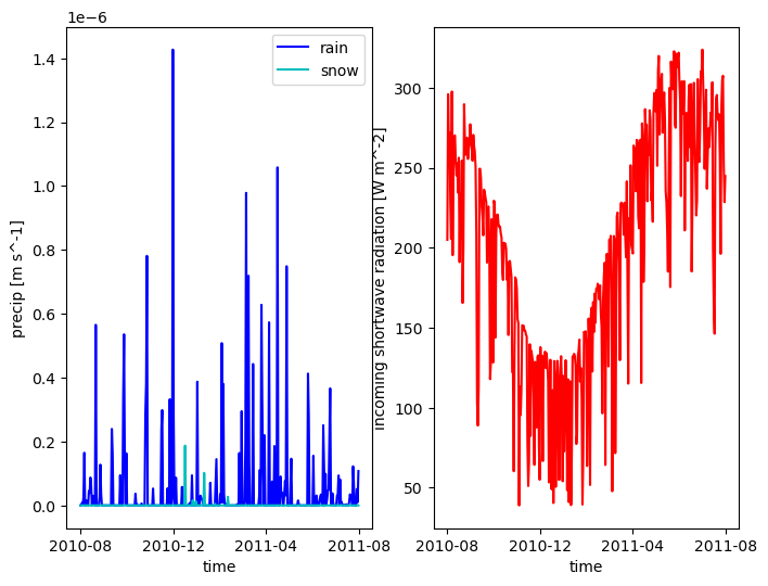
# write transient data to disk
filename = toOutput(f'{name}_aorc-{start.year}-{end.year}.h5')
output_filenames['meteorology_transient'] = filename
watershed_workflow.io.writeDatasetToHDF5(
    filename,
    met_data_transient
    )

2025-08-29 17:34:54,519 - root - INFO: Writing HDF5 file: /home/ecoon/code/watershed_workflow/repos/master/examples/Coweeta/output_data/Coweeta_aorc-2010-2014.h5

# compute the typical year
# note that we have to do this only on no-leap data to line up the days
#
# also, we do this on the original variables and then re-compute ATS quantities
ndays = met_data_warped['APCP_surface'].shape[0]
print('nyears = ', ndays // 365)
print('n days leftover = ', ndays % 365)
print('note, that leftover day(s) are leap day(s).')

nyears =  4
n days leftover =  1
note, that leftover day(s) are leap day(s).

# cannot compute a typical year for leap year -- need to align days-of-the-year
# remove leap day (Dec 31 of leap years)
met_data_noleap = watershed_workflow.data.filterLeapDay(met_data_warped)
met_data_noleap

# then compute a "typical" year
met_data_typical = watershed_workflow.data.computeAverageYear(met_data_noleap, 'time', 2010, nyears_cyclic_steadystate)

# and lastly convert to ATS
met_data_typical_ats = watershed_workflow.meteorology.convertAORCToATS(met_data_typical)

2025-08-29 17:34:55,346 - root - INFO: Converting AORC to ATS met input

# plot a few of the met data -- does it look reasonable?
plotMetData(met_data_typical_ats)

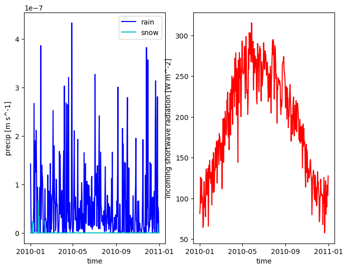
# write cyclic steadystate data to disk
filename = toOutput(f'{name}_daymet-CyclicSteadystate.h5')
output_filenames['meteorology_cyclic_steadystate'] = filename
watershed_workflow.io.writeDatasetToHDF5(
    filename,
    met_data_typical_ats,
    met_data_typical_ats.attrs)

2025-08-29 17:34:55,464 - root - INFO: Writing HDF5 file: /home/ecoon/code/watershed_workflow/repos/master/examples/Coweeta/output_data/Coweeta_daymet-CyclicSteadystate.h5

# compute the average precip rate for steadystate solution
precip_mean = (met_data_transient['precipitation rain [m s^-1]'].data + met_data_transient['precipitation snow [m SWE s^-1]'].data).mean()
logging.info(f'Mean precip value = {precip_mean}')

2025-08-29 17:34:55,976 - root - INFO: Mean precip value = 5.502343508705227e-08

Write ATS input files

Now we have the mesh file written and all of the forcing datasets (meteorology, LAI) written. It remains to write ATS XML files that will be the runs.

There are three runs done:

• steadystate: forces a surface + subsurface only problem with constant, uniform precip until true steadystate

• cyclic steadystate: forces with a typical year of averaged data

• transient: runs with real daily data from start to end

# Note that each of these are defined as functions so we can reuse them for all three input files.

# add the subsurface and surface domains
#
# Note this also adds a "computational domain" region to the region list, and a vis spec 
# for "domain"
def add_domains(main_list, mesh, surface_region='surface', snow=True, canopy=True):
    ats_input_spec.public.add_domain(main_list, 
                                 domain_name='domain', 
                                 dimension=3, 
                                 mesh_type='read mesh file',
                                 mesh_args={'file':mesh})
    if surface_region:
        main_list['mesh']['domain']['build columns from set'] = surface_region    
    
        # Note this also adds a "surface domain" region to the region list and a vis spec for 
        # "surface"
        ats_input_spec.public.add_domain(main_list,
                                domain_name='surface',
                                dimension=2,
                                mesh_type='surface',
                                mesh_args={'surface sideset name':'surface'})
    if snow:
        # Add the snow and canopy domains, which are aliases to the surface
        ats_input_spec.public.add_domain(main_list,
                                domain_name='snow',
                                dimension=2,
                                mesh_type='aliased',
                                mesh_args={'target':'surface'})
    if canopy:
        ats_input_spec.public.add_domain(main_list,
                                domain_name='canopy',
                                dimension=2,
                                mesh_type='aliased',
                                mesh_args={'target':'surface'})

def add_land_cover(main_list):
    # next write a land-cover section for each NLCD type
    for index, nlcd_name in zip(nlcd_indices, nlcd_labels):
        ats_input_spec.public.set_land_cover_default_constants(main_list, nlcd_name)

    land_cover_list = main_list['state']['model parameters']['land cover types']
    # update some defaults for
    # ['Other', 'Deciduous Forest']
    # note, these are from the CLM Technical Note v4.5
    #
    # Rooting depth curves from CLM TN 4.5 table 8.3
    #
    # Note, the mafic potential values are likely pretty bad for the types of van Genuchten 
    # curves we are using (ETC -- add paper citation about this topic).  Likely they need
    # to be modified.  Note that these values are in [mm] from CLM TN 4.5 table 8.1, so the 
    # factor of 10 converts to [Pa]
    #
    # Note, albedo of canopy taken from CLM TN 4.5 table 3.1
    land_cover_list['Deciduous Forest']['rooting profile alpha [-]'] = 6.0
    land_cover_list['Deciduous Forest']['rooting profile beta [-]'] = 2.0
    land_cover_list['Deciduous Forest']['rooting depth max [m]'] = 10.0
    land_cover_list['Deciduous Forest']['capillary pressure at fully closed stomata [Pa]'] = 224000
    land_cover_list['Deciduous Forest']['capillary pressure at fully open stomata [Pa]'] = 35000 * .10
    land_cover_list['Deciduous Forest']['albedo of canopy [-]'] = 0.1

# add soil sets: note we need a way to name the set, so we use, e.g. SSURGO-MUKEY.
def soil_set_name(ats_id):
    return subsurface_props_used.loc[ats_id, 'name']

def add_soil_properties(main_list):
    # add soil material ID regions, porosity, permeability, and WRMs
    for ats_id in subsurface_props_used.index:
        props = subsurface_props_used.loc[ats_id]
        set_name = soil_set_name(ats_id)
        
        if props['van Genuchten n [-]'] < 1.5:
            smoothing_interval = 0.01
        else:
            smoothing_interval = 0.0
        
        ats_input_spec.public.add_soil_type(main_list, set_name, ats_id, output_filenames['mesh'],
                                            float(props['porosity [-]']),
                                            float(props['permeability [m^2]']), 1.e-7,
                                            float(props['van Genuchten alpha [Pa^-1]']),
                                            float(props['van Genuchten n [-]']),
                                            float(props['residual saturation [-]']),
                                            float(smoothing_interval))    

# get an ATS "main" input spec list -- note, this is a dummy and is not used to write any files yet
def get_main(steadystate=False):
    main_list = ats_input_spec.public.get_main()

    # add the mesh and all domains
    mesh = os.path.join('..', output_filenames['mesh'])
    add_domains(main_list, mesh)

    # add labeled sets
    for ls in m3.labeled_sets:
        ats_input_spec.public.add_region_labeled_set(main_list, ls.name, ls.setid, mesh, ls.entity)
    for ss in m3.side_sets:
        ats_input_spec.public.add_region_labeled_set(main_list, ss.name, ss.setid, mesh, 'FACE')
    
    # add land cover
    add_land_cover(main_list)

    # add soil properties
    add_soil_properties(main_list)
        
    # add observations for each subcatchment
    if steadystate:
        time_args = {'cycles start period stop':[0,10,-1],}
    else:
        time_args = None
    ats_input_spec.public.add_observations_water_balance(main_list, "computational domain", 
                                                        "surface domain", "external sides",
                                                        time_args=time_args)

    return main_list

def populate_basic_properties(xml, main_xml):
    """This function updates an xml object with the above properties for mesh, regions, soil props, and lc props"""
    # find and replace the mesh list
    xml.replace('mesh', asearch.child_by_name(main_xml, 'mesh'))

    # find and replace the regions list
    xml.replace('regions', asearch.child_by_name(main_xml, 'regions'))

    # update the observations list
    obs = next(i for (i,el) in enumerate(xml) if el.get('name') == 'observations')
    xml[obs] = asearch.child_by_name(main_xml, 'observations')

    # update all model parameters lists
    xml_parlist = asearch.find_path(xml, ['state', 'model parameters'], no_skip=True)
    for parlist in asearch.find_path(main_xml, ['state', 'model parameters'], no_skip=True):
        try:
            xml_parlist.replace(parlist.getName(), parlist)
        except aerrors.MissingXMLError:
            xml_parlist.append(parlist)

    # update all evaluator lists
    xml_elist = asearch.find_path(xml, ['state', 'evaluators'], no_skip=True)
    for elist in asearch.find_path(main_xml, ['state', 'evaluators'], no_skip=True):
        try:
            xml_elist.replace(elist.getName(), elist)
        except aerrors.MissingXMLError:
            xml_elist.append(elist)    
    
    # find and replace land cover
    mp_list = asearch.find_path(xml, ['state', 'model parameters'], no_skip=True)
    lc_list = asearch.find_path(main_xml, ['state', 'model parameters', 'land cover types'], no_skip=True)
    
    try:
        mp_list.replace('land cover types', lc_list)
    except aerrors.MissingXMLError:
        mp_list.append(lc_list)

For the first file, we load a spinup template and write the needed quantities into that file, saving it to the appropriate run directory. Note there is no DayMet or land cover or LAI properties needed for this run. The only property that is needed is the domain-averaged, mean annual rainfall rate. We then take off some for ET (note too wet spins up faster than too dry, so don’t take off too much…).

def write_spinup_steadystate(name, precip_mean, **kwargs):
    # create the main list
    main = get_main()

    # set precip to 0.6 * the mean precip value
    precip = main['state']['evaluators'].append_empty('surface-precipitation')
    precip.set_type('independent variable constant', ats_input_spec.public.known_specs['evaluator-independent-variable-constant-spec'])
    precip['value'] = float(precip_mean * .6)

    
    # load the template file
    prefix = 'steadystate'
    xml = aio.fromFile(toInput(f'{prefix}-template.xml'))
    
    # update the template xml with the main xml generated here
    main_xml = ats_input_spec.io.to_xml(main)
    populate_basic_properties(xml, main_xml, **kwargs)

    # write to disk
    output_filenames[f'ats_xml_{prefix}'] = toWorkingDir(f'{name}-{prefix}.xml')
    filename = output_filenames[f'ats_xml_{prefix}']
    aio.toFile(xml, filename)

    # create a run directory
    output_filenames[f'ats_rundir_{prefix}'] = toWorkingDir(f'{name}-{prefix}')
    rundir = output_filenames[f'ats_rundir_{prefix}']
    os.makedirs(rundir, exist_ok=True)

For the second file, we load a transient run template. This file needs the basics, plus DayMet and LAI as the “typical year data”. Also we set the run directory that will be used for the steadystate run.

For the third file, we load a transient run template as well. This file needs the basics, DayMet with the actual data, and we choose for this run to use the MODIS typical year. MODIS is only available for 2002 on, so if we didn’t need 1980-2002 we could use the real data, but for this run we want a longer record.

def write_transient(name, cyclic_steadystate=False, **kwargs):
    # make a unique name based on options
    logging.info(f'Writing transient: {name}')

    if cyclic_steadystate:
        prefix = 'cyclic_steadystate'
        previous = 'steadystate'
    else:
        prefix = 'transient'
        previous = 'cyclic_steadystate'

    main = get_main()

    # add the DayMet evaluators
    if cyclic_steadystate:
        daymet_filename = output_filenames['meteorology_cyclic_steadystate']
    else:
        daymet_filename = output_filenames['meteorology_transient']
    ats_input_spec.public.add_daymet_box_evaluators(main, os.path.join('..', daymet_filename), True)

    # add the LAI filenames
    if cyclic_steadystate:
        lai_filename = output_filenames['nlcd_lai_cyclic_steadystate']
    else:
        lai_filename = output_filenames['nlcd_lai_transient']
    ats_input_spec.public.add_lai_point_evaluators(main, os.path.join('..', lai_filename), list(nlcd_labels_dict.values()))
    
    # load the template file
    template_filename = toInput(f'{prefix}-template.xml')
    xml = aio.fromFile(template_filename)

    # update the template xml with the main xml generated here
    main_xml = ats_input_spec.io.to_xml(main)
    populate_basic_properties(xml, main_xml, **kwargs)
    
    # update the start and end time -- would be nice to set these in main, but it would be 
    # confusing as to when to copy them in populate_basic_properties and when not to do so.
    start_day = 274
    if cyclic_steadystate:
        end_day = 274 + (nyears_cyclic_steadystate - 1) * 365 
    else:
        end_day = 274 + (end - start).days 
        
    par = asearch.find_path(xml, ['cycle driver', 'start time'])
    par.setValue(start_day)

    par = asearch.find_path(xml, ['cycle driver', 'end time'])
    par.setValue(end_day)
    
    # update the restart filenames
    for var in asearch.findall_path(xml, ['initial conditions', 'restart file']):
        var.setValue(os.path.join('..', output_filenames[f'ats_rundir_{previous}'], 'checkpoint_final.h5'))
   
    # write to disk and make a directory for running the run
    output_filenames[f'ats_xml_{prefix}'] = toWorkingDir(f'{name}-{prefix}.xml')
    filename = output_filenames[f'ats_xml_{prefix}']

    output_filenames[f'ats_rundir_{prefix}'] = toWorkingDir(f'{name}-{prefix}')
    rundir = output_filenames[f'ats_rundir_{prefix}']

    aio.toFile(xml, filename)
    os.makedirs(rundir, exist_ok=True)

write_spinup_steadystate(name, precip_mean)
write_transient(name, True)
write_transient(name, False)

/home/ecoon/code/ats/ats_input_spec/repos/master/ats_input_spec/io.py:43: UserWarning: Creating an incomplete XML object, missing entries!
  warnings.warn('Creating an incomplete XML object, missing entries!')
2025-08-29 17:34:56,105 - root - INFO: Writing transient: Coweeta
2025-08-29 17:34:56,123 - root - INFO: Writing transient: Coweeta

Completion and Summary

After this is complete, the following should work:

cd /path/to/ww/examples/Coweeta/Coweeta-steadystate
mpiexec -n 4 ats ../Coweeta-steadystate.xml &> out.log
cd ../Coweeta-cyclic_steadystate
mpiexec -n 4 ats ../Coweeta-cyclic_steadystate.xml &> out.log
cd ../Coweeta-transient
mpiexec -n 4 ats ../Coweeta-transient.xml &> out.log

# the following files were generated during this run:
print(f'{"role":<35}: filename')
print('-'*34, ': ', '-'*50)
for k,v in output_filenames.items():
    vs = list(splitPathFull(v))
    if vs[-2] == 'Coweeta':
        v2 = vs[-1]
    else:
        v2 = os.path.join(vs[-2], vs[-1])
    
    print(f'{k:<35}: {v2}')

role                               : filename
---------------------------------- :  --------------------------------------------------
modis_lai_transient                : output_data/Coweeta_LAI_MODIS_transient.h5
modis_lai_cyclic_steadystate       : output_data/Coweeta_LAI_MODIS_CyclicSteadystate.h5
nlcd_lai_cyclic_steadystate        : output_data/Coweeta_LAI_NLCD_CyclicSteadystate.h5
nlcd_lai_transient                 : output_data/Coweeta_LAI_NLCD_2010_2014.h5
subsurface_properties              : output_data/Coweeta_subsurface_properties.csv
mesh                               : output_data/Coweeta.exo
meteorology_transient              : output_data/Coweeta_aorc-2010-2014.h5
meteorology_cyclic_steadystate     : output_data/Coweeta_daymet-CyclicSteadystate.h5
ats_xml_steadystate                : Coweeta-steadystate.xml
ats_rundir_steadystate             : Coweeta-steadystate
ats_xml_cyclic_steadystate         : Coweeta-cyclic_steadystate.xml
ats_rundir_cyclic_steadystate      : Coweeta-cyclic_steadystate
ats_xml_transient                  : Coweeta-transient.xml
ats_rundir_transient               : Coweeta-transient

logging.info('this workflow is a total success!')

2025-08-29 17:34:56,168 - root - INFO: this workflow is a total success!