Soil Structural Data Comparison#
This notebook simply compares several different sets of soil structural data, clarifying how they can be used and noting their imperfections.
To run an integrated hydrology simulation, we need at least:
porosity
permeability
van Genuchten or other WRM, typically generated from Rosetta from texture data + bulk density
soil structural model (e.g. formations + horizons or other layering strategy)
For a structural model, we typically define two or three layers: bedrock, a geologic layer, and (sometimes) a soil layer. For the horizontal component, it is most convenient to work with formations – horizontal shapes whose bodies are assumed to be homogeneous within the shape and layer. We can work with fields of porosity and permeability, but currently ATS does not support fields of van Genuchten parameters, and running Rosetta at every pixel seems excessive anyway. So we prefer to avoid doing that.
# these can be turned on for development work
%load_ext autoreload
%autoreload 2
import watershed_workflow.ui
watershed_workflow.ui.setup_logging(1)
import numpy as np
from matplotlib import pyplot as plt

import watershed_workflow
import watershed_workflow.plot
import watershed_workflow.crs
import watershed_workflow.ui

import watershed_workflow.sources
# user input -- choose the HUC to work on
huc = '140200010204'
crs = watershed_workflow.crs.default_crs
# collect the HUCs from WBD
watershed = watershed_workflow.sources.ManagerWBD().getShapesByID([huc,], out_crs=crs)
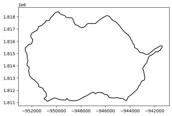
# plot what we have so far -- an image of the HUC
watershed.exterior.plot(color='k')
<Axes: >
watershed.crs
<Projected CRS: EPSG:5070>
Name: NAD83 / Conus Albers
Axis Info [cartesian]:
- X[east]: Easting (metre)
- Y[north]: Northing (metre)
Area of Use:
- name: United States (USA) - CONUS onshore - Alabama; Arizona; Arkansas; California; Colorado; Connecticut; Delaware; Florida; Georgia; Idaho; Illinois; Indiana; Iowa; Kansas; Kentucky; Louisiana; Maine; Maryland; Massachusetts; Michigan; Minnesota; Mississippi; Missouri; Montana; Nebraska; Nevada; New Hampshire; New Jersey; New Mexico; New York; North Carolina; North Dakota; Ohio; Oklahoma; Oregon; Pennsylvania; Rhode Island; South Carolina; South Dakota; Tennessee; Texas; Utah; Vermont; Virginia; Washington; West Virginia; Wisconsin; Wyoming.
- bounds: (-124.79, 24.41, -66.91, 49.38)
Coordinate Operation:
- name: Conus Albers
- method: Albers Equal Area
Datum: North American Datum 1983
- Ellipsoid: GRS 1980
- Prime Meridian: Greenwich
Available Products#
The following products are routinely available across the US (or globally).
GLHYMPS#
The Global Hydrogeology Maps product provides data by shapefile/formation, and provides:
porosity
permeability
depth-to-bedrock
This dataset is fairly complete, but there are some oddities – most notably much of the DTB field seems to be 0, and a significant subset of the porosity are 0 (mostly clays, we threshold at 1% to avoid this). But the data is pretty good and complete. However, it is missing WRM parameters (or equivalently, texture information).
# first let's look at GLYHMPS
# -- get the data
glhymps_mgr = watershed_workflow.sources.ManagerGLHYMPS()
gl = glhymps_mgr.getShapesByGeometry(watershed, out_crs=crs)
# convert it to standard ATS datasets
gl = watershed_workflow.soil_properties.mangleGLHYMPSProperties(gl)
gl
| ID | name | source | permeability [m^2] | logk_stdev [-] | porosity [-] | van Genuchten alpha [Pa^-1] | van Genuchten n [-] | residual saturation [-] | geometry | |
|---|---|---|---|---|---|---|---|---|---|---|
| 0 | 715383 | GLHYMPS-715383 | GLHYMPS | 6.309573e-16 | 2.50 | 0.19 | 0.000025 | 2.0 | 0.01 | MULTIPOLYGON (((-939257.031 1815576.693, -9392... |
| 1 | 715639 | GLHYMPS-715639 | GLHYMPS | 6.309573e-16 | 2.50 | 0.19 | 0.000025 | 2.0 | 0.01 | MULTIPOLYGON (((-941668.093 1811291.149, -9419... |
| 2 | 715707 | GLHYMPS-715707 | GLHYMPS | 1.000000e-13 | 2.00 | 0.22 | 0.000294 | 2.0 | 0.01 | MULTIPOLYGON (((-942876.044 1814661.915, -9427... |
| 3 | 715766 | GLHYMPS-715766 | GLHYMPS | 3.162278e-13 | 1.80 | 0.09 | 0.000817 | 2.0 | 0.01 | POLYGON ((-947358.28 1813697.645, -948118.709 ... |
| 4 | 715779 | GLHYMPS-715779 | GLHYMPS | 1.000000e-13 | 2.00 | 0.22 | 0.000294 | 2.0 | 0.01 | POLYGON ((-944025.909 1813309.319, -944527.763... |
| 5 | 715796 | GLHYMPS-715796 | GLHYMPS | 6.309573e-16 | 2.50 | 0.19 | 0.000025 | 2.0 | 0.01 | MULTIPOLYGON (((-933660.561 1797293.053, -9335... |
| 6 | 715833 | GLHYMPS-715833 | GLHYMPS | 3.162278e-13 | 1.80 | 0.09 | 0.000817 | 2.0 | 0.01 | MULTIPOLYGON (((-945234.306 1808748.423, -9451... |
| 7 | 726604 | GLHYMPS-726604 | GLHYMPS | 6.309573e-16 | 2.50 | 0.19 | 0.000025 | 2.0 | 0.01 | MULTIPOLYGON (((-941747.425 1812754.645, -9418... |
| 8 | 726608 | GLHYMPS-726608 | GLHYMPS | 6.309573e-16 | 2.50 | 0.19 | 0.000025 | 2.0 | 0.01 | MULTIPOLYGON (((-953864.501 1813999.085, -9542... |
| 9 | 726639 | GLHYMPS-726639 | GLHYMPS | 3.162278e-13 | 1.80 | 0.09 | 0.000817 | 2.0 | 0.01 | POLYGON ((-948778.786 1815596.524, -948024.977... |
| 10 | 726642 | GLHYMPS-726642 | GLHYMPS | 1.000000e-13 | 2.00 | 0.22 | 0.000294 | 2.0 | 0.01 | MULTIPOLYGON (((-944367.697 1813260.89, -94452... |
| 11 | 726650 | GLHYMPS-726650 | GLHYMPS | 6.309573e-16 | 2.50 | 0.19 | 0.000025 | 2.0 | 0.01 | MULTIPOLYGON (((-941147.259 1799041.493, -9410... |
| 12 | 726664 | GLHYMPS-726664 | GLHYMPS | 1.000000e-13 | 2.00 | 0.22 | 0.000294 | 2.0 | 0.01 | POLYGON ((-952109.643 1813503.499, -951346.338... |
| 13 | 726667 | GLHYMPS-726667 | GLHYMPS | 3.162278e-13 | 1.80 | 0.09 | 0.000817 | 2.0 | 0.01 | POLYGON ((-940163.504 1810040.228, -940089.924... |
| 14 | 726671 | GLHYMPS-726671 | GLHYMPS | 3.162278e-13 | 1.80 | 0.09 | 0.000817 | 2.0 | 0.01 | POLYGON ((-951971.487 1811058.543, -952225.723... |
| 15 | 730801 | GLHYMPS-730801 | GLHYMPS | 3.019952e-11 | 1.61 | 0.01 | 0.023953 | 2.0 | 0.01 | POLYGON ((-945003.907 1820005.317, -944742.248... |
# -- print extent of properties
gl_logK = np.log10(gl['permeability [m^2]'][:])
print('logK', gl_logK.min(), gl_logK.max())

poro = gl['porosity [-]']
print('poro', poro.min(), poro.max())
logK -15.2 -10.52
poro 0.01 0.22
gl.crs
<Projected CRS: EPSG:5070>
Name: NAD83 / Conus Albers
Axis Info [cartesian]:
- X[east]: Easting (metre)
- Y[north]: Northing (metre)
Area of Use:
- name: United States (USA) - CONUS onshore - Alabama; Arizona; Arkansas; California; Colorado; Connecticut; Delaware; Florida; Georgia; Idaho; Illinois; Indiana; Iowa; Kansas; Kentucky; Louisiana; Maine; Maryland; Massachusetts; Michigan; Minnesota; Mississippi; Missouri; Montana; Nebraska; Nevada; New Hampshire; New Jersey; New Mexico; New York; North Carolina; North Dakota; Ohio; Oklahoma; Oregon; Pennsylvania; Rhode Island; South Carolina; South Dakota; Tennessee; Texas; Utah; Vermont; Virginia; Washington; West Virginia; Wisconsin; Wyoming.
- bounds: (-124.79, 24.41, -66.91, 49.38)
Coordinate Operation:
- name: Conus Albers
- method: Albers Equal Area
Datum: North American Datum 1983
- Ellipsoid: GRS 1980
- Prime Meridian: Greenwich
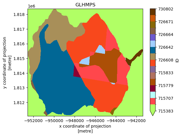
# -- color a raster by the polygons to see the structure
gl_color = watershed_workflow.data.rasterizeGeoDataFrame(gl, 'ID', 10)
gl_color = gl_color.rio.clip(watershed.geometry, watershed.crs)
# plot the formations
plt.figure()
unique_inds, gl_cmap, gl_norm, gl_ticks, gl_labels = \
       watershed_workflow.colors.createIndexedColormap(gl['ID'])


gl_color.plot.imshow(cmap=gl_cmap, norm=gl_norm)

plt.title("GLHMPS")
Text(0.5, 1.0, 'GLHMPS')
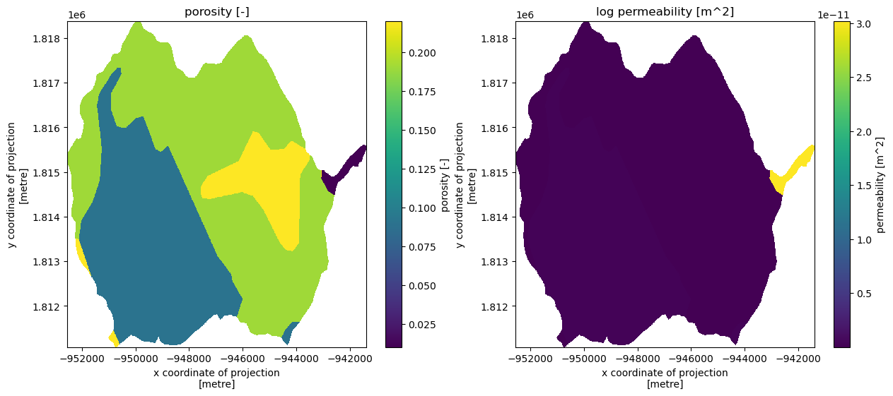
# generate glhymps porosity, permeability fields
# -- porosity
gl_poro = watershed_workflow.data.rasterizeGeoDataFrame(gl, 'porosity [-]', 10, nodata=np.nan)
gl_poro = gl_poro.rio.clip(watershed.geometry, watershed.crs)

# -- permeability
gl_perm = watershed_workflow.data.rasterizeGeoDataFrame(gl, 'permeability [m^2]', 10, nodata=np.nan)
gl_perm = gl_perm.rio.clip(watershed.geometry, watershed.crs)
# plot porosity and perm for glhymps
fig, axs = plt.subplots(1,2, figsize=(15,6))
gl_poro.plot.imshow(ax=axs[0])
gl_perm.plot.imshow(ax=axs[1])

axs[0].set_title('porosity [-]')
axs[1].set_title('log permeability [m^2]')
Text(0.5, 1.0, 'log permeability [m^2]')
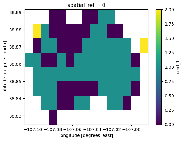
Pelletier et al (2016)#
In Pelletier et al 2016, a global depth-to-bedrock raster was developed. This has provided a reliable source for data about deep bedrock.
Pelletier, Jon D., et al. “A gridded global data set of soil, intact regolith, and sedimentary deposit thicknesses for regional and global land surface modeling.” Journal of Advances in Modeling Earth Systems 8.1 (2016): 41-65.
pell_mgr = watershed_workflow.sources.ManagerPelletierDTB()
pell = pell_mgr.getDataset(watershed.geometry[0], watershed.crs)['band_1']
pell = pell.rio.clip(watershed.to_crs(pell.rio.crs).geometry)

print(pell)
<xarray.DataArray 'band_1' (y: 8, x: 15)> Size: 480B
array([[nan, nan, nan,  0.,  0., nan, nan,  0.,  0.,  1.,  1., nan, nan,
        nan, nan],
       [nan,  2.,  1.,  0.,  0.,  0.,  0.,  0.,  1.,  1.,  0.,  0., nan,
        nan, nan],
       [nan,  0.,  1.,  1.,  0.,  0.,  0.,  1.,  1.,  1.,  1.,  1.,  1.,
        nan,  2.],
       [ 1.,  1.,  0.,  0.,  1.,  0.,  1.,  1.,  1.,  1.,  1.,  1.,  1.,
         0., nan],
       [nan,  1.,  1.,  1.,  1.,  1.,  1.,  1.,  1.,  1.,  1.,  1.,  1.,
         1., nan],
       [nan,  1.,  1.,  1.,  0.,  0.,  0.,  0.,  0.,  1.,  1.,  1.,  1.,
         0., nan],
       [nan, nan,  1.,  1.,  0.,  0.,  1.,  1., nan, nan,  1.,  1.,  0.,
        nan, nan],
       [nan, nan, nan,  0., nan, nan, nan, nan, nan, nan, nan, nan, nan,
        nan, nan]], dtype=float32)
Coordinates:
  * x            (x) float64 120B -107.1 -107.1 -107.1 ... -107.0 -107.0 -107.0
  * y            (y) float64 64B 38.89 38.88 38.87 38.86 38.85 38.85 38.84 38.83
    spatial_ref  int64 8B 0
Attributes:
    DataType:       Generic
    AREA_OR_POINT:  Area
    scale_factor:   1.0
    add_offset:     0.0
# plot Pelletier DTB
fig, ax = plt.subplots(1, 1)
pell.plot.imshow(ax=ax)
<matplotlib.image.AxesImage at 0x7907aeac1e50>
SSURGO#
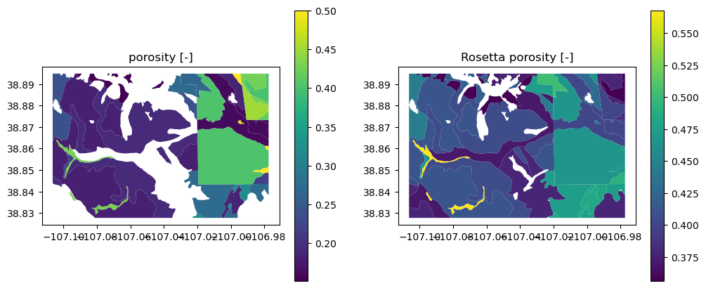
The NRCS’s SSURGO/STATSGO products provide shape-based information about the top 2m of soil. This data is provided by formation, and includes multiple formations (map-units), in which each map unit has (potentially) multiple components and each component has (potentially) multiple horizons. Short of taking the most prevelant component, we must average, so we tend to average horizons and components and just apply this uniformly in the top 2m. Provided include a complete set of parameters:
porosity
permeability
bulk density
texture
and more…
Unfortunately, while map units seem to cover the area of interest, they don’t all have at least one horizon with valid data, so some formations end up with NaN values. So while SSURGO can be used as an “overlay” with good soil layer information, it cannot be used alone without a gap-filling plan.
# ssurgo
nrcs_mgr = watershed_workflow.sources.ManagerNRCS()
nrcs = nrcs_mgr.getShapesByGeometry(watershed.geometry[0], watershed.crs)
nrcs
| mukey | geometry | residual saturation [-] | Rosetta porosity [-] | van Genuchten alpha [Pa^-1] | van Genuchten n [-] | Rosetta permeability [m^2] | thickness [m] | permeability [m^2] | porosity [-] | bulk density [g/cm^3] | total sand pct [%] | total silt pct [%] | total clay pct [%] | source | ID | name | |
|---|---|---|---|---|---|---|---|---|---|---|---|---|---|---|---|---|---|
| 0 | 498185 | POLYGON ((-107.01831 38.88358, -107.01841 38.8... | 0.240269 | 0.502882 | 0.000092 | 1.319916 | 3.617805e-13 | 1.520000 | 2.279759e-13 | 0.265563 | 1.207632 | 32.946001 | 24.529703 | 42.524296 | NRCS | 498185 | NRCS-498185 |
| 1 | 498188 | MULTIPOLYGON (((-106.98182 38.84868, -106.9821... | 0.208965 | 0.466656 | 0.000035 | 1.493607 | 3.227897e-13 | 0.710000 | 8.149200e-13 | 0.500000 | 1.230000 | 9.857377 | 66.027869 | 24.114754 | NRCS | 498188 | NRCS-498188 |
| 2 | 498205 | MULTIPOLYGON (((-106.98136 38.8663, -106.98188... | 0.181598 | 0.399993 | 0.000139 | 1.457559 | 4.938634e-13 | 1.520000 | 2.734080e-12 | 0.159737 | 1.413553 | 63.518421 | 22.988158 | 13.493421 | NRCS | 498205 | NRCS-498205 |
| 3 | 498206 | MULTIPOLYGON (((-106.9782 38.87179, -106.97836... | 0.181598 | 0.399993 | 0.000139 | 1.457559 | 4.938634e-13 | 1.520000 | 2.734080e-12 | 0.159737 | 1.413553 | 63.518421 | 22.988158 | 13.493421 | NRCS | 498206 | NRCS-498206 |
| 4 | 498208 | MULTIPOLYGON (((-106.98546 38.87211, -106.9855... | 0.208316 | 0.428990 | 0.000071 | 1.420938 | 2.830658e-13 | 1.520000 | 1.184189e-12 | 0.185986 | 1.302697 | 40.662797 | 38.201188 | 21.136015 | NRCS | 498208 | NRCS-498208 |
| 5 | 498209 | MULTIPOLYGON (((-106.9777 38.86864, -106.97773... | 0.208316 | 0.428990 | 0.000071 | 1.420938 | 2.830658e-13 | 1.520000 | 1.184189e-12 | 0.185986 | 1.302697 | 40.662797 | 38.201188 | 21.136015 | NRCS | 498209 | NRCS-498209 |
| 6 | 498218 | POLYGON ((-106.98706 38.8434, -106.98621 38.84... | 0.239708 | 0.491429 | 0.000080 | 1.336891 | 3.047481e-13 | 1.520000 | 1.822373e-13 | 0.217763 | 1.227697 | 29.210470 | 30.763761 | 40.025768 | NRCS | 498218 | NRCS-498218 |
| 7 | 498231 | MULTIPOLYGON (((-107.01992 38.86516, -107.0199... | 0.213285 | 0.466663 | 0.000059 | 1.416784 | 3.782943e-13 | 1.070000 | 7.331979e-13 | 0.403218 | 1.197010 | 32.639846 | 41.078960 | 26.281194 | NRCS | 498231 | NRCS-498231 |
| 8 | 509477 | MULTIPOLYGON (((-107.08069 38.82938, -107.0808... | 0.175133 | 0.567740 | 0.000103 | 1.383180 | 2.438575e-12 | 1.520000 | 3.039095e-12 | 0.428779 | 0.807465 | 62.072368 | 17.973684 | 19.953947 | NRCS | 509477 | NRCS-509477 |
| 9 | 509479 | MULTIPOLYGON (((-106.99601 38.8277, -106.99586... | 0.230885 | 0.378365 | 0.000079 | 1.374540 | 1.031721e-13 | 1.250000 | 3.172415e-12 | NaN | 1.524444 | 39.279352 | 38.916498 | 21.804150 | NRCS | 509479 | NRCS-509479 |
| 10 | 509481 | MULTIPOLYGON (((-107.10589 38.83252, -107.1043... | 0.230885 | 0.378365 | 0.000079 | 1.374540 | 1.031721e-13 | 1.250000 | 3.172415e-12 | NaN | 1.524444 | 39.279352 | 38.916498 | 21.804150 | NRCS | 509481 | NRCS-509481 |
| 11 | 509482 | MULTIPOLYGON (((-107.09255 38.83101, -107.0931... | 0.207877 | 0.369886 | 0.000092 | 1.397760 | 1.474479e-13 | 1.205000 | 4.654687e-12 | NaN | 1.530585 | 45.389069 | 37.890283 | 16.720648 | NRCS | 509482 | NRCS-509482 |
| 12 | 509513 | MULTIPOLYGON (((-107.10611 38.87963, -107.1058... | 0.219597 | 0.445168 | 0.000072 | 1.395746 | 2.727324e-13 | 1.520000 | 9.122162e-13 | 0.237423 | 1.280039 | 38.422252 | 35.742028 | 25.835720 | NRCS | 509513 | NRCS-509513 |
| 13 | 509514 | MULTIPOLYGON (((-107.00249 38.83035, -107.0020... | 0.241801 | 0.474101 | 0.000079 | 1.340429 | 2.435161e-13 | 1.520000 | 2.375523e-13 | 0.271630 | 1.274496 | 30.592982 | 31.535307 | 37.871711 | NRCS | 509514 | NRCS-509514 |
| 14 | 509529 | MULTIPOLYGON (((-107.06282 38.87776, -107.0629... | 0.196811 | 0.356163 | 0.000157 | 1.406091 | 2.260935e-13 | 1.520000 | 5.850942e-12 | NaN | 1.607097 | 63.571711 | 22.369079 | 14.059211 | NRCS | 509529 | NRCS-509529 |
| 15 | 509532 | MULTIPOLYGON (((-107.08446 38.83002, -107.0851... | 0.199783 | 0.412306 | 0.000087 | 1.422578 | 2.966015e-13 | 1.520000 | 1.526682e-12 | 0.182238 | 1.356006 | 47.934946 | 34.134907 | 17.930147 | NRCS | 509532 | NRCS-509532 |
| 16 | 509544 | MULTIPOLYGON (((-107.04457 38.87875, -107.0457... | NaN | NaN | NaN | NaN | NaN | 1.520000 | 7.000000e-15 | NaN | NaN | NaN | NaN | NaN | NRCS | 509544 | NRCS-509544 |
| 17 | 509547 | MULTIPOLYGON (((-107.06405 38.865, -107.06431 ... | NaN | NaN | NaN | NaN | NaN | 1.520000 | 4.230700e-11 | NaN | 2.030000 | NaN | NaN | NaN | NRCS | 509547 | NRCS-509547 |
| 18 | 509548 | MULTIPOLYGON (((-107.04607 38.82944, -107.0456... | 0.189314 | 0.404765 | 0.000104 | 1.433685 | 3.617371e-13 | 1.520000 | 2.006536e-12 | 0.193350 | 1.379123 | 53.676535 | 31.072368 | 15.251096 | NRCS | 509548 | NRCS-509548 |
| 19 | 509559 | MULTIPOLYGON (((-107.06648 38.88147, -107.0667... | 0.210870 | 0.420608 | 0.000078 | 1.410010 | 2.516507e-13 | 0.618125 | 7.504374e-13 | 0.151250 | 1.341513 | 43.240132 | 35.652961 | 21.106908 | NRCS | 509559 | NRCS-509559 |
| 20 | 509561 | POLYGON ((-107.09952 38.8459, -107.09969 38.84... | 0.246665 | 0.467696 | 0.000081 | 1.332817 | 2.088819e-13 | 1.396471 | 1.590777e-13 | 0.218625 | 1.305591 | 30.228443 | 31.026630 | 38.744927 | NRCS | 509561 | NRCS-509561 |
| 21 | 509567 | POLYGON ((-107.00507 38.8277, -107.00534 38.82... | 0.242574 | 0.482738 | 0.000079 | 1.336289 | 2.612348e-13 | 1.520000 | 1.748267e-13 | 0.186440 | 1.257167 | 28.780573 | 31.506579 | 39.712848 | NRCS | 509567 | NRCS-509567 |
| 22 | 509571 | MULTIPOLYGON (((-107.01403 38.8277, -107.01549... | 0.245090 | 0.481450 | 0.000081 | 1.330972 | 2.469105e-13 | 1.520000 | 1.517041e-13 | 0.319721 | 1.269125 | 28.517802 | 30.887384 | 40.594814 | NRCS | 509571 | NRCS-509571 |
| 23 | 509577 | MULTIPOLYGON (((-107.0234 38.83592, -107.02335... | NaN | NaN | NaN | NaN | NaN | 1.520000 | NaN | NaN | NaN | NaN | NaN | NaN | NRCS | 509577 | NRCS-509577 |
| 24 | 509726 | POLYGON ((-106.9774 38.88088, -106.97741 38.88... | 0.169567 | 0.356505 | 0.000202 | 1.548169 | 5.589350e-13 | 1.520000 | 5.317991e-12 | 0.399396 | 1.586579 | 73.750000 | 17.539474 | 8.710526 | NRCS | 509726 | NRCS-509726 |
| 25 | 509733 | POLYGON ((-106.98406 38.87324, -106.98641 38.8... | 0.157366 | 0.400499 | 0.000221 | 1.762072 | 1.819618e-12 | 0.860000 | 5.262229e-12 | 0.449752 | 1.423158 | 82.200000 | 9.300000 | 8.500000 | NRCS | 509733 | NRCS-509733 |
| 26 | 509739 | POLYGON ((-106.98875 38.88562, -106.98912 38.8... | 0.180715 | 0.378278 | 0.000162 | 1.471752 | 4.414571e-13 | 0.510000 | 1.286655e-12 | 0.425230 | 1.506585 | 67.256098 | 20.512195 | 12.231707 | NRCS | 509739 | NRCS-509739 |
| 27 | 509789 | MULTIPOLYGON (((-106.97834 38.88014, -106.9784... | 0.184149 | 0.372988 | 0.000140 | 1.438542 | 3.199534e-13 | 1.520000 | 2.504075e-12 | 0.427204 | 1.515197 | 60.823026 | 26.676974 | 12.500000 | NRCS | 509789 | NRCS-509789 |
| 28 | 509794 | POLYGON ((-106.9774 38.8732, -106.98227 38.873... | 0.220962 | 0.383130 | 0.000140 | 1.367408 | 2.004353e-13 | 1.520000 | 1.554090e-12 | 0.415245 | 1.545395 | 60.571711 | 18.441447 | 20.986842 | NRCS | 509794 | NRCS-509794 |
| 29 | 708040 | POLYGON ((-106.99643 38.8811, -106.99801 38.88... | NaN | NaN | NaN | NaN | NaN | NaN | NaN | NaN | NaN | NaN | NaN | NaN | NRCS | 708040 | NRCS-708040 |
| 30 | 3084845 | POLYGON ((-106.99416 38.8712, -106.99463 38.87... | 0.214182 | 0.444803 | 0.000063 | 1.416842 | 2.920197e-13 | 1.520000 | 6.113237e-13 | 0.476856 | 1.263443 | 35.464974 | 40.343256 | 24.191769 | NRCS | 3084845 | NRCS-3084845 |
# plot ssurgo porosity, note white inside the domain is NaN values
fig, axs = plt.subplots(1,2, figsize=(12,5))

nrcs.plot('porosity [-]', ax=axs[0], legend=True)
axs[0].set_title('porosity [-]')
nrcs.plot('Rosetta porosity [-]', ax=axs[1], legend=True)
axs[1].set_title('Rosetta porosity [-]')
Text(0.5, 1.0, 'Rosetta porosity [-]')
import matplotlib.colors as mpc
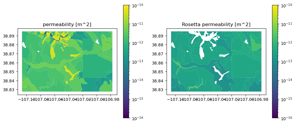
# plot ssurgo porosity, note white inside the domain is NaN values
fig, axs = plt.subplots(1,2, figsize=(12,5))
nrcs.plot('permeability [m^2]', ax=axs[0], legend=True,
norm=mpc.LogNorm(vmin=1e-16, vmax=1e-10))
axs[0].set_title('permeability [m^2]')
nrcs.plot('Rosetta permeability [m^2]', ax=axs[1], legend=True,
norm=mpc.LogNorm(vmin=1e-16, vmax=1e-10))
axs[1].set_title('Rosetta permeability [m^2]')
Text(0.5, 1.0, 'Rosetta permeability [m^2]')
SoilGrids (2017)#
SoilGrids includes 250m, global rasters of:
depth to bedrock
bulk density
texture via percent sand/silt/clay
and more…
Effectively everything is available that is needed to run Rosetta to get a full suite of parameters. Vertically, bulk density and texture information are provided at 7 layers, the deepest starting at 2m. Data is complete globally, and doesn’t seem to have much missing data except under water bodies. The only downside is the raster nature of the data – to use this directly we would have to run every pixel through Rosetta and provide fields of Van Genuchten parameters. We could conceivably use the rasters of porosity and permeability, but it seems more convenient to work by formation instead of as a raster.
Note that here we use the 2017 product instead of the 2020 product as that has yet to include depth-to-bedrock. The depth-to-bedrock here seems fairly inaccurate – generally we have stopped using SoilGrids for this reason.
Therefore we keep this section here in case anyone wants to play with this product, but comment it out.
# SoilGrids
#
# NOTE: this may not work any more -- we may need to deprecate SoilGrids.
#sg_mgr = watershed_workflow.sources.ManagerSoilGrids2017()
#sg = sg_mgr.getDataset(watershed)


#print(sg)
SoilGrids has holes where there is standing water, but we still need soil in these places. Fill these using a nearest neighbor algorithm.